COMP 130
Elements of Algorithms and Computation
Spring 2012
![[Rice University]](http://www.staff.rice.edu/images/staff/branding/shield.jpg)
Last lecture, we ended with the notion of "conditional probability", which are probabilities of events relative to a subset of the overall universe of possibilities. The problem is that we often do not have easy access to the actual conditional probability we desire. In fact, a common situation is that instead of P(A|B), we actually have the exact opposite, P(B|A). Let's illustrate the issue with an example:
Consider a medical test for some dastardly but relatively rare disease -- take your pick, cancer of the whatever, Alzheimer's, Parkinson's, etc., it doesn't matter because the same issues apply. Such tests are not-infallible, so their accuracy is described in terms of 4 inter-related percentages or probabilities:
Note that the sum of the True-Positive and False-Positive probabilities must be one, since if the person has the disease, then the test will register something: 1 = P(pos|hasDisease)+P(neg|hasDisease). Likewise, the sum of the True-Negative and False-Negative probabilities must also add up to one: 1 = P(neg|noDisease)+P(pos|noDisease). This means that technically, there are really only 2 independent probabilities here, one from True/False-Positive and one from True/False-Negative.
These probabilities are the ones that are measured because they naturally fall out of a clinical trial: You have a group of test patients that you know have the disease and give them the test and record the number of positive results divided by the number of test patients -- this gives your the True-Positive probability. Then you take a group of test patients that you know do not have the disease and give them the test as well. The number of positive test results will give you the False-Negative probability.
Unfortunately for already-stressed-out patients, none of the above probabilities is the one that concerns them. The question that patients who receive a positive test result want answered is "what is the probability that I have the disease, given that I just received a positive test result?", i.e. P(hasDisease|pos), which is the exact opposite of the True-Positive conditional probability!
If the medical test is "95% accurate", i.e. the True-Probability is 95%, or P(pos|hasDisease) = 0.95, does this mean that the test results indicate that there is only a 1 in 20 chance that the patient will luck out and escape the ravages of that disease?
Not so fast. Let's take a more careful look at the situation and the actual P(hasDisease|pos) conditional probability that the patient is interested in. For the sake of drama only, let's consider a rare disease, one which only afflicts a relatively small percentage of the population, say 2.5% of the population. Here are some reasonable test performance measures to work with:
We can represent the situation with the following scaled Venn diagram where the green areas represent the percentage of the population of people that don't have the disease (97.5%) while the yellow areas represent the percentage of the people that actually do have the disease (2.5%). The accuracy of the medical test for the disease is represented by the red striped portions of the diagram. The yellow+red stripe area is 95% of the yellow area, representing the 95% True-Positive rate of the test. The green+red stripe area is 10% of the green area, representing the 10% False-Positive rate of the test.
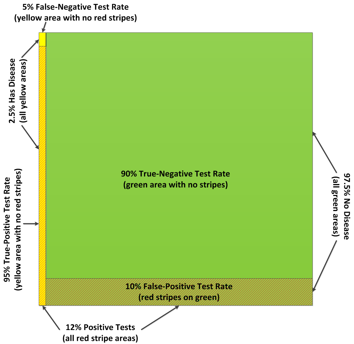
The red stripe areas thus represent to percentage of the population that would receive a positive test result, either as a True-Positive or a False-Positive result. To calculate this area, we first calculate the individual areas:
The area of the True-Positive results is the intersection of the positive results and hasDisease regions:
P(pos ∩ hasDisease) = P(pos|hasDisease)*P(hasDisease) = 0.95*0.025 = 0.02375.
The area of the False-Positive results is the intersection of the positive results and noDisease regions:
P(pos ∩ noDisease) = P(pos|noDisease)*P(noDisease) = 0.10 * 0.975 = 0.0975.
The area of the Positive results is thus the sum of the two above areas:
P(pos) = P(pos ∩ hasDisease)+ P(pos ∩ noDisease) = P(pos|hasDisease)*P(hasDisease) + P(pos|noDisease) = 0.02375 + 0.0975 = 0.12125.
Notice that the majority of the contribution to this value comes from the False-Positives, not the True-Positives!
The desired quantity, the probability of having the disease given a positive test result is thus the ratio of the True-Positive area to the overall Positive area:
P(hasDisease|pos) = P(pos ∩ hasDisease)/P(pos) = P(pos|hasDisease) * P(hasDisease)/P(pos) = 0.02375/0.12125 = 0.1958.
That is, the positive test result really means that the patient has only about a 1 in 5 chance of having the disease, not 19 in 20! Whew!
Why did this happen? The point here that P(pos|hasDisease)and P(hasDisease|pos) fundamentally measure two different things. P(pos|hasDisease)measures the ratio of the yellow-striped area to the total yellow area, i.e. the percentage of positive test results in the reduced world where everyone has the disease. On the other hand, the patient has been thrust into a world where all tests are positive, which is not the same world as the True-Positive scenario, because in the patient's world, not everyone has the disease. On the Venn diagram the sub-world where all tests are positive is all the red-striped areas. P(hasDisease|pos) is thus the ratio of the yellow-striped area to the total striped area.
Our dramatic results are due to the fact that we chose a rare disease. This means that a 95% test accuracy with regards to people who definitely have disease amounts to a number of people that is actually smaller than the number of people that get one of the 10% False-Positive results from the 97.5% remaining disease-free population. That is, the rarity of the disease combined with the non-zero False-Positive rate lead to a situation where the False-Positives actually outnumbered the True-Positives.
Not to throw cold water on our medical sigh of relief, but it should be pointed out that in some sense the test has done its job because our probability of having the disease has risen from 2.5% before taking the test, up to 20% after the test is performed and returns a positive result. That's a factor of 8 more sure of having the disease. Bummer...
Class Question: How does one's probability of not having the disease change from before taking the test to after getting a negative result from taking the test?
Let's take another look at the last equation above:
P(hasDisease|pos) = P(pos|hasDisease) * P(hasDisease)/P(pos)
Notice that it has a very interesting property: A conditional probably can be calculated in terms of its inverse conditional property!
That is, P(hasDisease|pos) is related to P(pos|hasDisease)by the ratio of their pieces: P(hasDisease)/P(pos)
In the year 1763, 2 years after his death, it was revealed to the Royal Society in England that the Reverend Thomas Bayes had formulated a generalization of the above observation, hereto be known as "Bayes' Theorem":
P(A|B) =
P(B|A) * P(A)/P(B) This formula seems innocuous enough, but we will see that there is much more to it than meets the eye... |
 Thomas Bayes (1701-1761) |
See another example of using Bayes' Theorem, using playing cards.
Let's back up for a moment and consider other interpretations a conditional probability, P(A|B). first, let's consider the notion of the probability of something as a "degree of belief" in that something. That is, a "probability of being" something. One way to think of the conditional probability is that since it represents the relative occurance of A in the reduced world of B, we can rephrase that by saying "P(A|B) is the belief in A given the evidence of B". Above, the patient is trying to gauge their belief that they have the disease given the evidence of the positive test result.
Let's re-arrange and color-code our example's formula and Bayes' Theorem to help us interpret what is going on:
P(hasDisease|pos) = P(hasDisease) * P(pos|hasDisease)/P(pos)
P(A|B) = P(A) * P(B|A)/P(B)
Compare the various parts of the equations:
P(A) is called the "prior", because it is the probability of something, hasDisease or A, with no conditions, i.e. the probability of the desired entity, in terms of the full universe of possibilities.
P(A|B), on the other hand, is a conditional probability of the same entity as P(A), but with regards to reduced world of positive test results or B. In other words, P(A), the original degree of probability of (i.e. the belief in) an outcome with regards to the entire universe, has been altered by a multiplicative factor (the blue parts of the equations) to create a new belief in the same outcome under new considerations, namely a positive test result or B. This new, altered belief/probability is called the "posterior".
The blue part of the equation tells us how the experiment, i.e. the conditional imposed on the system, affects the prior probabilities to transform them into their new, constrained universe.
P(B|A) is called the "likelihood" because it represents how likely it is to observe the evidence that was seen. In our example, this is the True-Positive rate, which tells us how accurate the test is when administered to a known diseased patient.
P(B) is called the "model evidence" or "marginal likelihood" and defines the reduced world as defined by operation of the general behavior of the experiment, in our example, the medical test's positive result behavior on both diseased and undiseased test subjects. This is the overall probability of a particular consideration being used to modify the probability of the prior, e.g. the probability of a positive test result across the entire population.
Models
There is one more thing to note and that is the role of the probability of diseased and non-diseased people in the world in general. As pointed out, the dramatic results of our example were due in large part to the creation of a world where the probability of having the disease in the world was very much smaller than the probability of not having the disease. If you think about the issue, you will realize that the utility of the medical test depends on knowing the occurrence of the disease in the general population but in order to determine that occurrence, one has to use the medical test. In some ways, we have a circular argument here!
The bottom line is that the value of the occurrence of the disease in the general population (universe) must come from outside this analysis system, i.e. for the purposes of this analysis, the probabilities of having or not having the disease in the general population are assumptions. In other words, those probabilities form a model of reality we under which we perform our analysis.
Bayes Theorem represents the transformation of a prior degree of belief in an outcome by the inclusion of experimental evidence as represented by likelihoods and underlying model(s).
A model divides the universe in a particular manner, cutting it up into a description as a collection of smaller pieces, e.g. has disease or no disease. An experiment also divides the universe into smaller pieces, but in different directions than the model. Performing an experiment and getting a specific result has effectively leaves a smaller, distorted model.
The process of using Bayes Theorem to try to decide what outcome, here whether the patient does or does not actually have the disease, based on known, invariant properties of the system, the medical test accuracy data, the experimental results, here the medical test, and underlying models, the probabilities of diseased and non-diseased people in general, is called Bayesian inference
Generalization to more than 2 priors and 2 likelihoods
Moving to a system with more than 2 priors simply means that there are more possibilities in terms of the desired outcomes that one wants. None of the math actually changes. We've simply divided our initial universe into more than 2 pieces. Likewise, having more than 2 likelihoods simply means that we can't automatically calculate the other likelihood by simply subtracting one likelihood from 1. We have to explicitly calculate each likelihood, that's all.
In terms of inferring our result, life is not black-and-white anymore. Before, with only 2 choices, saying the probability of having the disease, given a positive test, is 20% is also tantamount to saying that the probability of not having the disease, given a positive test, is 100% - 20% = 80%. If we have multiple possibilities, we simply have to calculate each one and go with the most probable outcome.
Bayesian Inference Process
| Step: | Example: |
| 1. Construct a model of the world, i.e. the probabilities of the priors. | Create the probabilities of having or not having the disease |
| 2. Devise an experiment | Create the medical test |
| 3. Get performance data on the experiment, i.e. the likelihoods. | Using known priors from the model, i.e. people known to have or not have the disease, obtain the True-Positive and False-Positive rates for the medical test. This step is often called the "training step" because you are training your system to be able to perform inferences by building up a set of likelihoods (conditional probabilities that divide the universe in a different manner than the priors). |
| 4. Calculate the marginal likelihoods. | Calculate the probabilities of postive and negative test results across the entire population (universe). |
| 5. Given a particlar experimental outcode, calculate the posteriors for all the possible priors. | For a positive test result, calculate P(hasDisease|pos) and P(noDisease|pos). |
| 6. Choose the posterior with the highest probability as the most likely outcome. | For a positive test result, go with the patient does NOT have the disease. because that posterior, P(noDisease|pos) = 80%. |
See an example of Bayesian inference using digit recognition.
For a more complete and detailed treatment of Bayes' Theorem and Bayesian inference, please see Prof. Subramanian's lecture notes from Comp140:
Comp200 students: Part 2, Part 3 and Part 4.
Comp130 students: Part 2, Part 3 and Part 4.