Algorithm |
Multiplication |
Some of the classical applications of adaptive filters are system identifications, channel equalization, signal enhancement and signal prediction. Our proposed application is noise cancellation, which is a type of signal enhancement. The general case of such an application is depicted below.
Where the signal x(k) is corrupted by noise n1(k), and the signal n2(k) is correlated to the noise. When the algorithm converges, the output signal e(k) will be an enhanced version of the signal.
The Mean Square Error (F[e(k)] = [|E[e(k)|2]) is a quadratic function of the parameters of the weights. This property is important and is used in adaptive filters because it has only one universal minimum value. This means it is suitable for many types of adaptive algorithms, and will result in a decent convergence behavior. In contrast, IIR filters need more complex algorithms and analysis on this issue.
There are many adaptive algorithms that can be used in signal enhancement, such as the Newton algorithm, the steepest-descent algorithm, the Least-Mean Square (LMS) algorithm, and the Recursive Least-Square (RLS) algorithm. We chose to use the LMS algorithm because it is the least computationally expensive algorithm and provides a stable result.
2. Standard LMS
The equations below depict the LMS algorithm.
1. Filtering:
y(k) = XT(k)W(k)
2. Error estimation:
e(k) = d(k) - y(k)
3. Filter Tap weights update:
g(k)=2e(k)*x(k)
W(k+1) = W(k) + u*g(k)
Where k is the number of iterations of the algorithm, y(k) is the output of the filter, X(k) is the buffered input signal in vector form, W(k) is the filter tap weights in vector form, e(k) is the error between the desired (reference) signal d(k) and the filter's output y(k), u is the convergence factor (step size), and W(k+1) is the filter tap weights for the next iteration. In this algorithm, g(k) is an important value. It is the estimated gradient (partial differential of E[e2(k)] on the weight of a tap) or the projection of the square of the current error signal, e2(k) on the filter tap weight. When the algorithm converges, g(k) is expected to be a very small number with zero mean value.
The step-size (u) must be in the range 0 < u < 1/Lmax, where Lmax is the largest eigenvalue of R = E[X(k)TX(k)] (one of R's properties is that all eigenvalues of R should be non-negative real numbers). In practice, a much smaller u than 1/Lmax is recommended when Lmin is much smaller than Lmax. The minimum number of steps it takes this algorithm to converge is proportional to Lmax / Lmin.
The variable step-size LMS algorithm (VSLMS) is a variation on the LMS algorithm that uses a separate step-size for each filter tap weight, providing a much more stable and faster convergence behavior. The first two steps in the algorithm are the same as before, however the third step in updating the weights has changed as shown below.
3. Filter Tap weights and step-size update
For i = 0, 1, ..., N-1
gi(n) = e(n)x(n-i)
ui(n) = ui(n-1) + psign[gi(n)], sign[gi(n-1)]
if ui(n) > umax,
ui(n) = umax
if ui(n) < umin,
ui(n) = umin
wi(n+1) = wi(n) + 2 ui(n)gi(n)
End
Our initial plan was to implement the Variable Step-Size LMS algorithm described above. We performed simulations in MatLab to test the functionality of this algorithm for our application (8 taps) and the results were more than a little unsettling. We discovered that the algorithm would not converge even with the smallest value of u and with inputs that are exactly the same. This happens because we require normalization of the weight values if the step-size is very large, otherwise the values of the weights increase until they reach the highest possible value. In order to perform this normalization procedure we need several comparison operations and division operations, which is beyond the capacity of our chip.
In an attempt to find a simpler LMS algorithm that would work with our chip we looked at an alternative called the Sign-Sign LMS, which uses fixed step-size and the following equation for updating the weights:
wi(n+1) = wi(n) + 2 u * sign(gi(n))
This algorithm works well, but the drawback is that its u becomes the step of the weights, which results in an extremely slow convergence, approximately 3000 iterations on average.
In order to find a faster LMS algorithm that would work with our chip limitation we decided to look at the original LMS algorithm again and determine how we could perform some kind of normalization of the weight values. We performed a number of simulations on various input noise signals in order to obtain the Lmax (described in Section 2 above). We found Lmax to be in the range of 14,000 to 19,000. According to the convergence rule, any positive u less then 1/19000 should promise convergence. In actuality we have to choose a much smaller u because the Lmin of the noise signal can be very small. The step-size (u) that we found to be best in our simulation is 1/(2048*256), which is much smaller than the upper bound but provided the fastest convergence generating an acceptable output.
To implement this small step-size in our equation, we hide the value of the step-size in the gradient by normalizing the result of g = x * err. This is done in two steps. First we right shift g by 11 bits, leaving the 5 most significant bits (including sign bit), which is equivalent to dividing g by 2048. Second, we move the decimal point from after the least significant bit to before the most significant bit, which is equivalent to dividing by 256. This actually does not require any operation to be performed, we simply add this to the weight which is also just a fraction.
Our space on the target chip will allow us to represent x, d, and e with 8 bits in 2's complement format. Our w and u have to be 8-bit fixed point 2's complement numbers, where the decimal point is before the most significant bit, because the range of the weight is from -0.5 to 0.5 and should never get any larger or smaller.
5. Simulation
This section provides an overview of the final MatLab simulation model we used and the results we obtained. Figure 5.1 shows the overall system diagram with the noise input being fed into an FIR filter and the signal + noise input being compared with the output of the FIR filter to produce the error output.
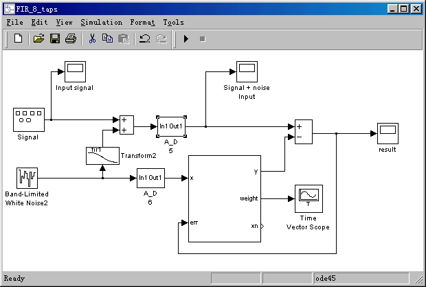
Figure 5.1 Our LMS System Simulation Model
Figure 5.2 below unveils the adaptive FIR filter block shown above. This depicts the 8 taps in the filter. For each tap, there is another sub-model shown in Figure 5.3 that updates the weight value for that tap depending on the X input and Error input. Y is calculated using the previously stored value for each of the filter tap weights.
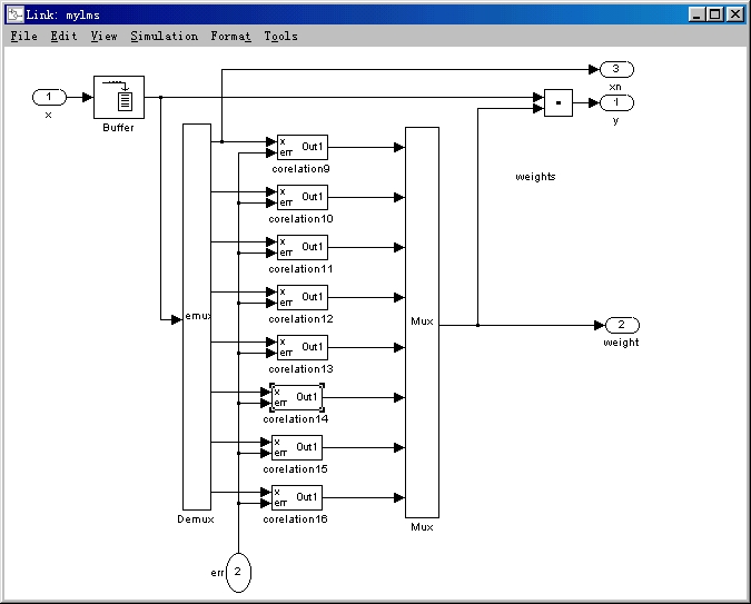
Figure 5.2 FIR Filter Simulation Model
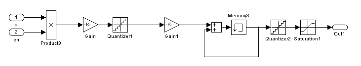
Figure 5.3 Weight Update Simulation Model
Figure 5.4 below depicts the results from running the simulation model shown above with a white noise input signal and a sine wave input signal. The topmost graph on the right labeled Signal + noise input is the desired signal and the middle graph on the right is the error output or result of the filter. As you can see, the noise has been almost completely cancelled and the output signal is similar to the input sine wave. The large graph on the left shows the value of each of the 8 weights after convergence ( ~ 600 iterations). As you can see, the values for each of the weights are never larger than 0.5 and never drops below -0.5. In addition to the simulation results shown below, we have simulated our system with variations on the noise input and have not seen any problems. We have not yet simulated our system with an actual voice and noise input because the version of MatLab on UNIX only supports this in Windows, and we have not been able to obtain a copy of MatLab to run in Windows with this feature. As soon as we get a version with this feature or another program that has this feature we will perform this simulation with real input signals.
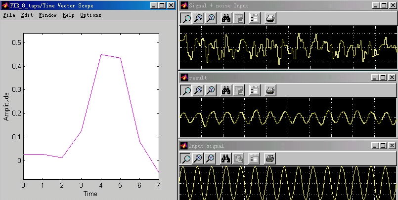
Figure 5.4 Simulation Results