Dynamic Programming

Dynamic programming is an algorithmic technique often utilized to efficiently compute solutions to optimization problems. (The use of the word “programming” in this context is an older use meaning constructing tables, not “the act of creating programs” as we more often define it today.) Dynamic programming is similar to the divide and conquer strategies we have seen so far in that it partitions the given problem into smaller subproblems and then combines their solutions to compute a global solution; however, in the cases where dynamic programming is used the partitioned subproblems are generally not independent (that is that some subproblems may overlap with other subproblems or subproblems may share subproblems). A divide and conquer approach to such a problem runs the risk of repeatedly solving these common subproblems again and again in a wasteful manner. Dynamic programming approaches avoid this problem by ensuring that repeated subproblems are solved only once and that those solutions are leveraged at each repeated point of the subproblem's occurence with the computation.

Assembly-line Scheduling - A candidate problem

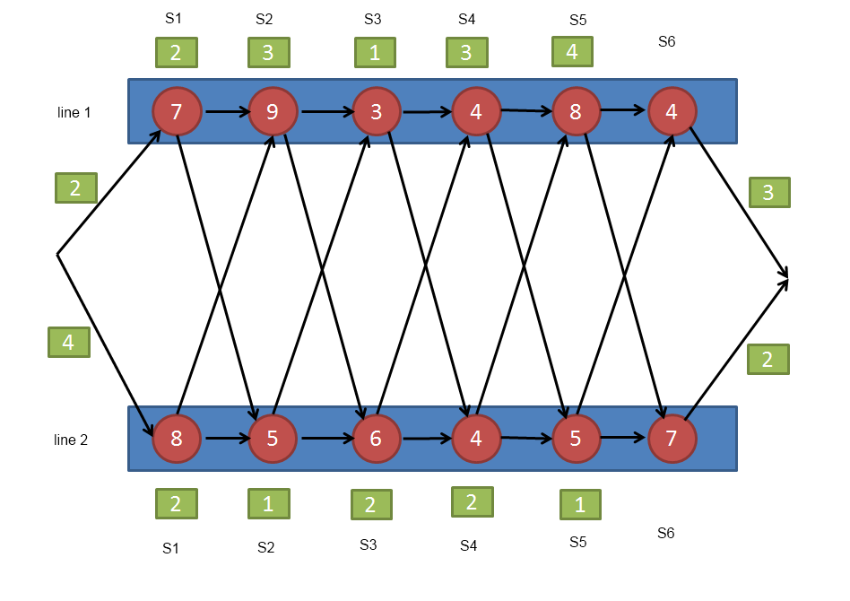
Consider the case of the Banana Computing company. Banana has recently announced the availability of the their latest personal computing device, the iPeel. Due to overwhelming demand, Banana (along with their partner, Houndconn) has constructed a new factory devoted to constructing iPeels. The factory contains two parallel assembly lines organized into stations, where each station is responsible for one aspect of iPeel construction:

(example shamelessly borrowed from Introduction to Algorithms 2nd edition by Cormen et al., page 325.)

Each station on either assembly line (for example, station 3 on assembly line 1 and station 3 on assembly line 2) performs the same task. However, the stations differ in the amount of time required to perform their task due to slight variations in the the construction of the manufacturing equipment. The time required to perform a task at each station is shown in the red circle representing that station. Full construction of an iPeel requires manufacturing from each of the six stations. Normally an iPeel starts at S1 on one of the assembly lines and proceeds through all six steps on that same assembly line. Optionally however, an iPeel may removed from one assembly line after completing station n and placed at station n+1 on the alternate assembly line (for example, one station on an assembly line may be turned off for maintenance.) The time required to transplant an iPeel from one assembly line to the other for each station is shown in the green box above that station. For example, after completing manufacturing at S5 on assembly line 1, an iPeel can be transferred to S6 on assembly line 2 in 4 time units. It also requires time to move all the iPeel parts from storage to each assembly line (shown by the green boxes to the left of the lines) and more time to box and store the final product as they come off each assembly line (shown by the green boxes to the right of the assembly line.)

Question: If a single special order came in on a weekend when the plant was inactive, what is the fastest way to move a single iPeel through the construction sequence?

Can we develop a recursive algorithm to solve this problem?

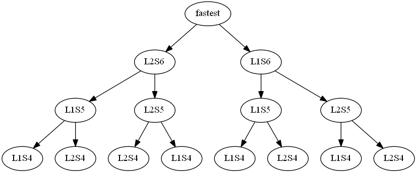
In the recursive solution, we see that the same instance of several subproblems occur again and again and are solved again and again. Recomputing the solution to the exact same subproblem in the recursive solution is wasteful.

Dynamic Programming: A different approach

We will attempt to avoid the wasteful recomputation of the recursive solution by instead using a bottom up DP strategy. Our general strategy is to create a lookup table that will store the minimum time required from manufacturing start to the completion of LnSm as we discover what that minimum time is. As the algorithm progresses, should we ever need this minimum time value we can consult our lookup table instead of recomputing the solution. We will progressively consider each each station in ascending order for both lines (e.g. L1S1, L2S1, L1S2, L2S2 ...) and compute the minimum completion time of a station leveraging the knowledge of the minimum completion time of all previous stations. Once the minimum times are know for L1S6 and L2S6 we can compute the minimum possible time of the entire manufacturing process.

Minimum Time Table: each entry in the table represents the minimum time cost from start to the completion of that entry's station by any possible path.

Step 1: Fill in the Minimum Time table for the first stations L1S1 and L2S1.

The minimum completion time to complete S1 from either line is easily derived from the problem statement. It is simply the time cost of manufacturing at that station plus the time cost of moving material to that station:

Step 2-6:

While unknown stations still exist, use the known information about the minimum time costs of L1Sn and L2Sn to compute the minimum time cost of both L1Sn+1 and L2Sn+1. It is in this step that the dynamic programming technique comes into play. When computing L1Sn+1 and L2Sn+1 each computation will require knowledge of both L1Sn and L2Sn. This is an example of how, in this problem, subproblem overlap occurs. However, by consulting the lookup table instead of performing an explicit computation for these identical subproblems, we can reuse solutions in our dynamic programming strategy to improve algorithmic efficiency when compared to the recursive solution.

Exercises

Ex 1. Pseudocode for Minimum Time

Create pseudocode for an algorithm that uses dynamic programming to find the fastest path through the iPeel plant.

Ex 2. Time Complexity of DP

What is the time complexity of your algorithm?

Ex 3. Time Complexity of Recursive Solution

Give a tight bound (Theta) for the time complexity of the recursive algorithm discussed in lab.

Ex 4. Compute Minimum Time

Use the following Python representations of the problem data to create a function that uses the dynamic programming technique above to find the minimum time cost of constructing a single iPeel. Assert your result is 38.

startup_cost = { 1:2, 2:4 }
line_1_start_cost = startup_cost[1];

exit_cost = {1:3, 2:2 }
line_2_exit_cost = exit_cost[2]

manufacturing_cost = { (1, 1) : 7, (1, 2) : 9, (1, 3) : 3, (1, 4) : 4, (1, 5) : 8, (1,6) : 4,
                       (2, 1) : 8, (2, 2) : 5, (2, 3) : 6, (2, 4) : 4, (2, 5) : 5, (2,6) : 7 }
line2_station_3_mcost = manufacturing_cost[(2,3)]

transfer_cost = { ((1,1), (2,2)) : 2, ((1,2), (2,3)) : 3, ((1,3), (2,4)) : 1, ((1,4), (2,5)) : 3, ((1,5), (2,6)) : 4,
                  ((2,1), (1,2)) : 2, ((2,2), (1,3)) : 1, ((2,3), (1,4)) : 2, ((2,4), (1,5)) : 2, ((2,5), (1,6)) : 1 }
end_of_L2S3_to_start_of_L1S4_xfercost = transfer_cost[((2,3),(1,4))]

Ex 5. Fastest Path

Modify your solution to also compute the path of minimum cost. Assert your path is L1S1, L2S2, L1S3, L2S4, L2S5, L1S6.

---

Submit your code

At the end of lab, submit your group's Python code here.