|
General Form of Adaptive Filters
|
|
|
Pictured here is the general structure of an adaptive filter. The main points to be noted here are
- The system takes in two inputs
- The top box has one input
- The bottom box has that same input plus an error input
- The top box is being changed by the bottom box
- What's the output?
If the bottom box is the brain, then the top box is the body. The brain is using what it knows and putting it through an algorithm in which to control the body. The algorithm is always of the form
|
General Form of Algoritm for Updating Coefficients
|
|
|
The functions are determined by you, the programmer. Examples commonly used are LMS (Least Mean Squared), NLMS (Normed LMS), RMS (Root Mean Squared), and ABC (just kidding). We will use LMS for this project.
The user will want an output. Depending on what the system is for, the output will be either y(n), e(n), or the filter itself.
|
Adaptive Filter for FIR Filter Identification
|
|
|
The bottom two boxes are our adaptive system. It is figuring out what the top box is. The top box is a Finite Impluse Response (FIR) filter programmed by MATLAB with the magic command "filter(B,A,signal)." The filter is a "Direct Form II Transposed" implementation of the standard difference equation:
a(1)*y(n) = [b(1)*x(n) + b(2)*x(n-1) + ... + b(nb+1)*x(n-nb)] - [a(2)*y(n-1) + ... + a(na+1)*y(n-na)]
We simulated this filter with the command "filter(rand(3,1), 1, signal)" This sets a(1) in the difference equations to one. The first three B coefficients are given random numbers. That's what our adaptive filter is going to figure out. The rest of the coefficients are set to zero.
Now to put our boxes into action. As seen by the block diagram, any random is signal is fed into our system and the unknown filter. The signal is filtered through the unknown, and our initial guess of the unknown. The difference of the outputs (plus some noise) e(n) is taken and put through our magical coefficient updating algorithm to get our programmable digital filter closer to the unknown. As more signal is fed through, our digital filter will start to mimic the unknown. It's learning! (see the code archive for our MATLAB code)
|
Plots (click images for larger versions)
|
A
|
B
|
C
|
D
|
|
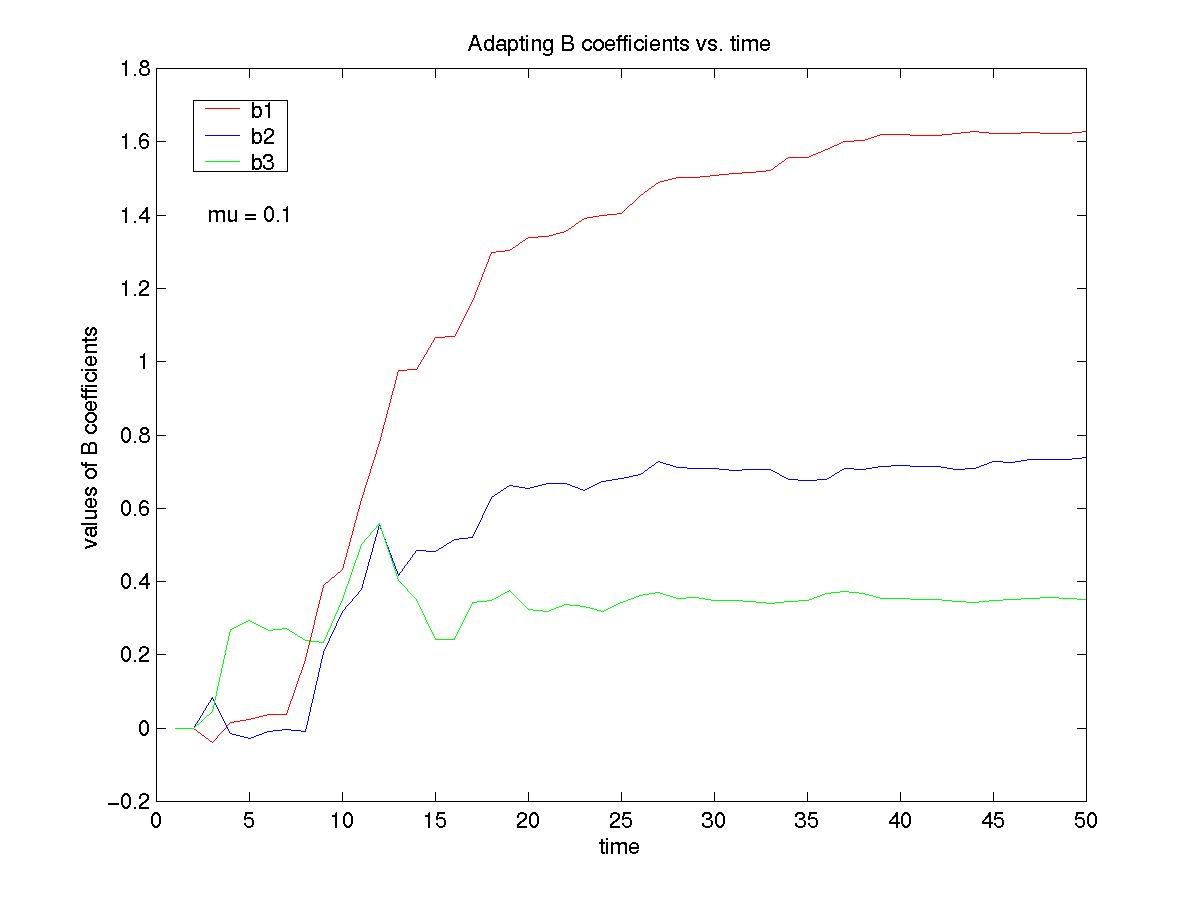
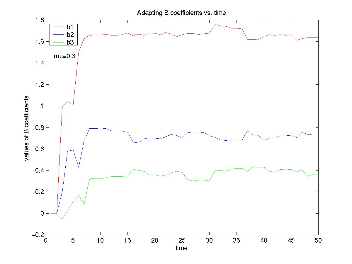
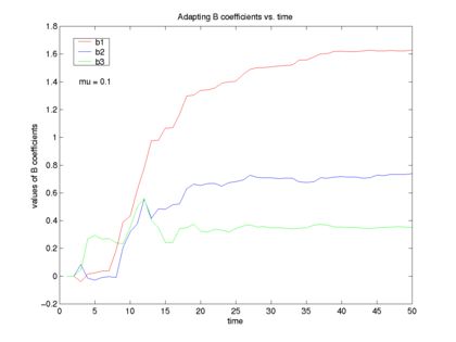
A) This is a plot of the coefficients of our adaptive filter vs. time. You can see the values converge to the unknown values. So now we know b(1)=1.65, b(2)=0.72, b(3)=0.38. We have our system identified.
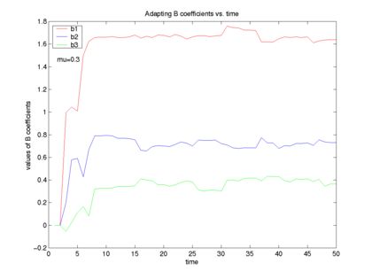
B) The first example had mu, the step size of our error correction, equal to 0.1. If we make it a little larger, say 0.3, we get faster convergence as seen here. But it we have mu too large, say 0.5, the system diverges.
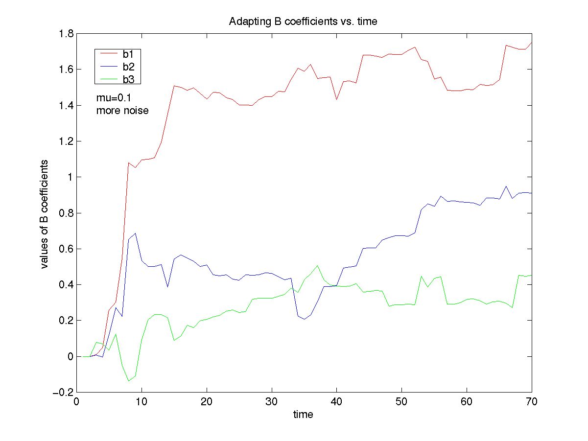
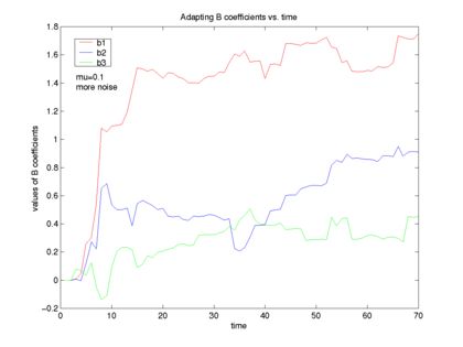
C) If we have the noise turned up, the adaptive filter will oscillate more, but we can still make out that it converges to an estimate of the B coefficients.
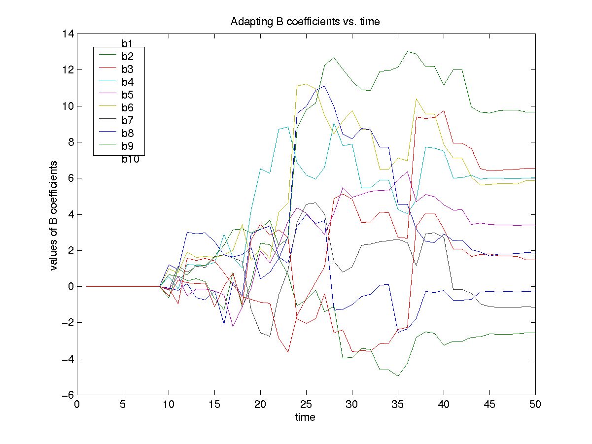
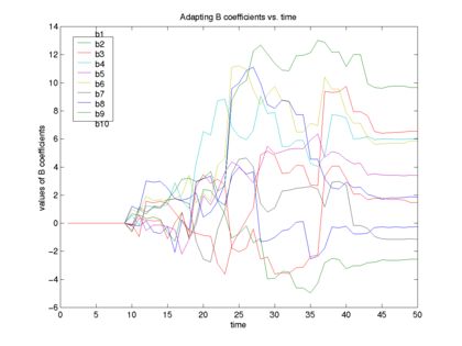
D) We can also figure out any n-order FIR filter. Here's a 10th order filter.
|
|
One of the most commmon practical applications of adaptive filters is
noise cancellation. We simulated the situation in which the adaptive filter
needed to remove a time varying noise from a desired speech signal. This
could be a model for a person speaking on a cell phone in a car where his
voice is corrupted by noise from the car's engine.
|
Block Diagram for Noise Cancellation
|
|
|
We begin with two signals, the primary signal and the reference
signal. The primary signal contains both our desired voice signal and the
noise signal from the car engine.
The reference signal is a tapped version of the noise in the primary
signal, i.e. it must be correlated to the noise
that we are trying to eliminate. In the case that we are trying to model,
the primary signal may come from a microphone at the speaker's mouth which
picks up both the speech signal and a noise signal from the car engine. The
reference signal may come from another microphone that is placed away from
the speaker and closer to the car engine, so the reference noise will be
similar to the noise in primary but perhaps with a different phase and
with some additional white noise added to it.
|
Reference: Estimation of Noise
|
|
|
The LMS algotrithm updates the filter coefficients to minimize the
error between the primary signal and the filtered noise. In the process of
pouring through some class notes from ELEC 431, we found that it can be
proven through some hard math that the voice component of the primary
signal is orthogonal to the reference noise. Thus the minimum this error can be
is just our desired voice signal.
We then experimented with varying different parameters. It turns out that
the output we get is very, very sensitive to mu. Apparently there is a very
precise method for finding the most optimal mu, something to do with the
eigenfuction of the correlation matrix between the primary and reference
signals, but we used an educated trial and error technique. Basically we
found that mu affects how fast a response we were able to get; a larger mu
gives a faster response, but with a mu that is too large, the result will
blow up.
We also experimented with several different filter lengths.
One question that is often asked is why we cannot simply subtract
the reference noise from the primary signal to obtain our desired voice
signal. This method would work well if the reference noise was exactly the
same as the actual noise in primary.
|
Reference Noise = Actual Noise
|
|
|
However, if the reference noise is
exactly 180 degrees out of phase the with noise in primary, the noise will
be doubled in the output. As can be seen in the figures below, the output
from the adaptive filter is still able to sucessfully cancel out the noise.
|
Reference Noise 180 deg Out-of-Phase from Actual Noise
|
|
|
|
Filtered Output - It still works!
|
|
|
The one important condition on the use of adative filters for noise
cancellation is that the noise can't be similar to the desired voice
signal. If this is the case, the error that the filter is trying to
minimize has the potential to go to zero, i.e. the filter also wipes out
the voice signal. The figure below shows the output of the adaptive filter
when the reference noise used was a sinusoid of the same frequency as that
of the voice signal plus some white noise.
|
Filtered Output - No Good When Voice = Noise
|
|
|