| |
|
|

Discrete Wavelet Decomposition
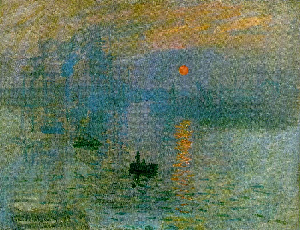
Looking at our base pictures we notice that some of the artists painted with a lot of localized
high frequency content. For example, Monet is typified by short, brisk strokes with no definite
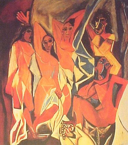
lines, which corresponds to a lot of high frequency content. On the other hand, Picasso used
planes of color and geometric shapes, which correspond to high frequency content only around the
edges of his planes. Hence, we thought it would be appropriate to try to distinguish between
the artists by getting a measure of the amount of high frequency content in their paintings.
The Discrete Wavelet Tranform
In order to analyze the amount of high frequency content in the image we used the two-dimensional discrete
wavelet transform (dwt2) as provided in the MATLAB Wavelet toolbox. The dwt2 command produces four matrices
of coefficients; the first contains the approximation coefficients, the second contains the wavelet coefficients
along the horizontal, the third matrix contains the vertical wavelet coefficients, and the fourth contains the
diagonal coefficients.
The following figure summarizes the dwt2 algorithm for computing the coefficients.
The dwt2 algorithm can also be applied again on the approximation coefficients hence allowing us to go
down a number of levels. Looking at the (one level) dwt2 decomposition of the paintings (below) our suspicions are
corroborated as we see that Monet exhibits much higher localized frequency throughout the painting in all
of the detail coefficients.
| One level Decomposition of Monet Sunrise: |
 |
 |
| |
| One level Decomposition of Picasso Les Mouses: |
 |
 |
The Besov Norm
In order to quantitatively compare two paintings we needed to attain a numerical measure of their high frequency
content. This is where our research led us to look into Besov norms, which provide us a way of quantifying this
information.
formula for calculating the Besov norm
 |
We found it most useful to take the Besov norm of each painting with p=1, hence we would just sum up the
absolute value of the coefficients in the different levels and then add the norm of the approximation coefficients
at the last level.
| Calculating the Besov norm of a three level DWT: |
| |
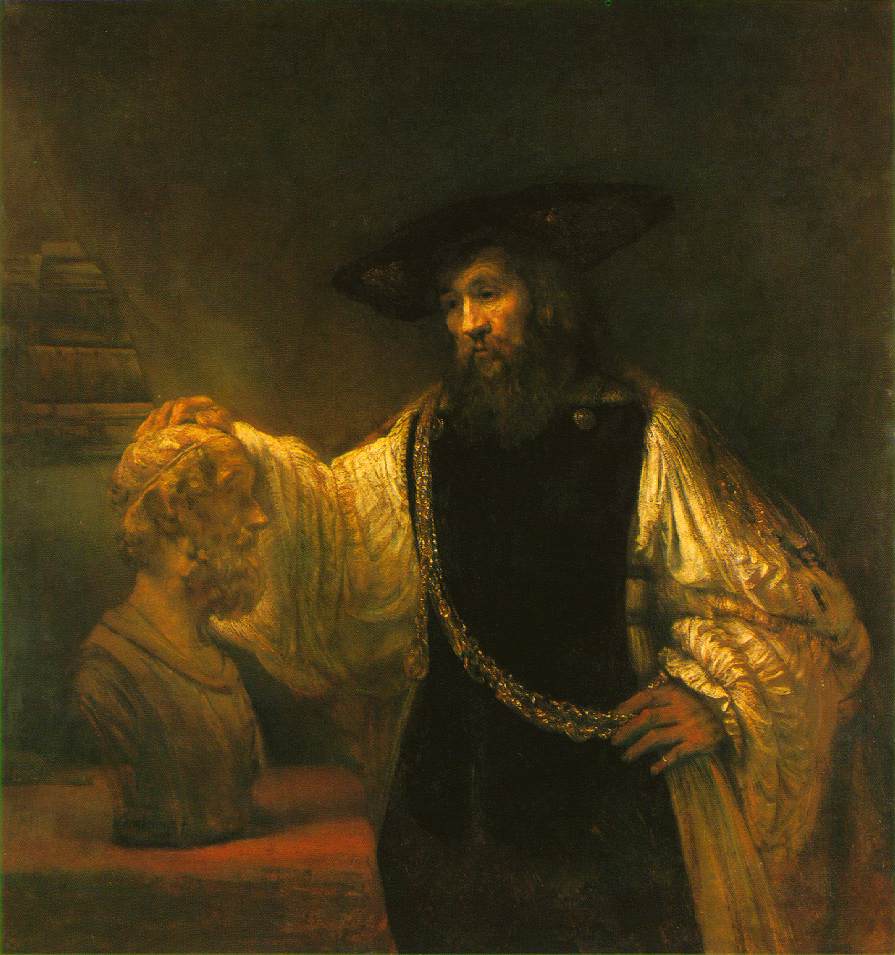
Here is an example of our
Rembrandt Aristotle-Homer with
the DWT applied 2 levels: |
 |
 |
 |
Results
Looking at the Besov norm of each of the artists we are able to see trends in their paintings. In particular, as
expected, Picasso exhibited a consistently lower norm than the other artists. Rembrandt, too, exhibited relatively
well-behaved norm values in his paintings, which were on average just above those of Picasso. Monet on the
other hand, exhibited a wide range of values and hence a clear trend was not evident from his paintings.
| Plot of picture number vs. Besov norm: |
| |
Although the Discrete Wavelet Decomposition along with Besov norm analysis showed us some trends between
two of the three artists, the trends of these particular artists overlapped. Consequently, even though we believe
this tool is very useful in analyzing paintings of different artists, we did not find this tool very useful in distinguishing between Monet, Rembrandt, and Picasso.
 DWT MATLAB code DWT MATLAB code

|
|
|