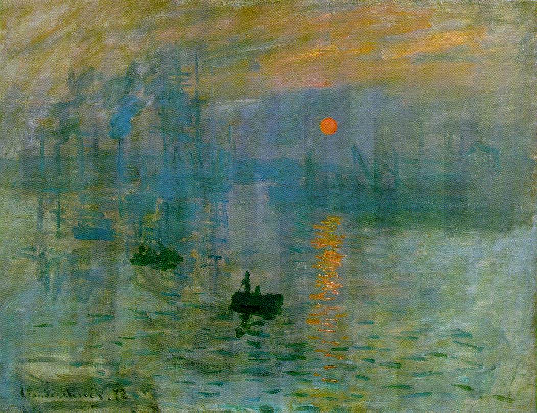
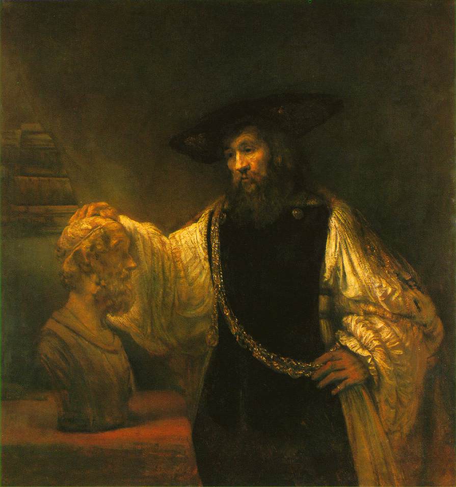
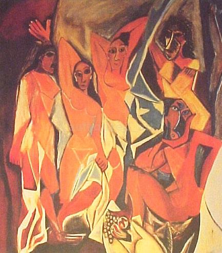
Edge detection proved to be a good tool to differentiate the artists from one another. Monet consisted of short rapid brushstrokes throughout. This gave an image with lots of variation in the entire picture. Rembrandt focused his pictures his subject while the rest of the picture was mostly black. Picasso used geometric shapes and planar colors to give only a few sharp edges where the shapes changed.
Trends
These characteristics transferred over to the edge plot where Monet had edges throughout his paintings, Rembrandt only where his subjects were (almost nothing in the background), and Picasso only on the edges of his geometric shapes. Of course these statements are a generalization, but they served to help see another difference between the artists.
Monet edge plot
Rembrandt edge plot
Picasso edge plot
The three pictures shown here are representative of each artist's
style and indicate how most of the edge plots looked like.
Summary of findings
artist
edge concentration
edge plot appearance
Monet
high
high frequencies throughout
Rembrandt
medium
concentrated high frequencies
Picasso
low
sparse geometric shapes
Algorithm:
The method used for the edge plot was the Sobel method that consisted of finding the maximum and the minimum of the derivative. Where the difference was greatest was considered an edge. This uses the total variation norm that consists of finding the integral of the derivative of the function. The Sobel method gave the best results for differentiating between the artists. The Laplacian method that low pass filters the image (with a Gaussian filter) and then finds the zero crossing gave a lot of noise and the low pass filter distorted the image. The Canny method (most recommended by MATLAB) that also takes into account the second derivative of the function gave too much noise as well.
To compile these findings into a solid number that can be compared across the board we added up the number of lines that were 8 pixels in length or longer (in a binary image). With a MATLAB function we could get a solid number out. Once again this method uses a change on the total variation method. To find the lines in our plot the program has to consider that not all lines are straight and many curve all over the plot. So the total variation norm has the capability to find the length of a line that is not straight. With these numbers we could see general trends with each artist.
It can be seen that Monet was almost always the highest and Picasso the lowest. Although Rembrandt jumped around between the two the fact that we could differentiate Monet and Picasso with almost complete certainty really helped our program. This was because Rembrandt was easily found from the other two by the darkness of his pictures.