This project was an open-ended attempt at sound compression. The MP3 technology was the guiding force for our project, but we did not implement all of its algorithms. We tried to emulate some of the principles of an MP3 and also tried some other ideas.

The first step was deciding on how to take a time-domain signal and take it to the frequency domain. Basically, we just used the Fast Fourier Transform and the Discrete Cosine Transform. Each was useful for different compression schemes. <Transforms>

We started out trying very simple ways to compress our signal. For example, we simply lowpass filtered it. The results were not very impressive; you basically made telephone quality sound out of CD quality sound with a compression of 80%. We wanted to try something fancier than that.

Another simple algorithm was to drop some magnitudes of an FFT such as every odd one. This gave equally unimpressive results, and the sound quality for the amount of compression is kind of random. <drop_odds.m>

One compression algorithm we came up with is the Average Energy Algorithm. Basically, we found the mean and standard deviation of the energy in the frequency domain. Then, we kept the frequencies which have energies between 1 standard deviation from the mean, 2 standard deviations from the mean, and 3 standard deviations from the mean. <Average Energy>

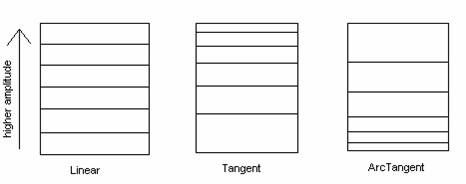
The next step was to introduce quantization. Quantization is an important way to compress analog data so that it can be stored digitally. Our source files were .wav files quantized at 16 bits per sample which we considered as being almost an analog input. We decided on three quantization schemes: linear, tangent, and arctangent. With linear quantization giving equal bits to all amplitudes, tangent giving more bits to higher amplitudes, and arctangent giving more bits to lower amplitudes. <Quantization> Below is a diagram of the quantization "buckets" for the three methods:

 

Next we started implementing some of the algorithms used by MP3s. The first had to do with the Psychoacoustic Model.

There are two frequency ranges that the human ear is more sensitive to: 1,000Hz - 5,100Hz and 12,500Hz - 15,200Hz. The first range corresponds to the human voice frequencies while the latter corresponds to high-pitch screeches. An example of how the human ear is more sensitive to these two ranges of frequencies is that we are actually more attentive to a baby crying than a washing machine running.

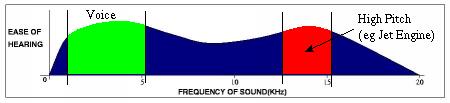
Courtesy of the Audio Tutorial site

First, we performed the DCT. Then, we quantized the signal in one of the three ways that we implemented. The basic idea is to give more bits to the frequencies in the ranges 1,000Hz - 5,100Hz and 12,500Hz - 15,200Hz. So we quantized those ranges with varying numbers of bits. <psycho.m>

After we did the quantization, we threw away frequencies that are either below 20Hz or above 20,000Hz since we cannot hear those frequencies anyway. Then, we took the inverse DCT and listened to the outputs.

Next we tried to implement masking. Masking is a phenomenon that occurs when loud and quiet signals are close together in time or frequency. We tried to implement masking in frequency. Read more:<Frequency Masking>

Finally, we tried simple windowing of the signal. We took the original time domain signal and broke it into smaller chunks. Then we performed the same operations on these chunks as before.