Analog Implementation

We began our work in the Elec lab, led by Tom "Ben is my Bitch" Miller, the analog guru of the group. The first filters we built and tested were passive first order filters. After those unaccustomed to the black magic of analog cursed and complained that the filters made no sense, we decided to use active analog filters instead.

Although the cost of active filters is higher (due to the use of an op-amp), there are several good reasons which justify the added cost and added complexity of design. Active filters can be designed for a gain of one (or more) while passive filters always have a gain of less than one. This can allow the filter to be inserted with no signal loss, or one could even combine the functions of filtering and amplification in one op-amp. In fact, capacitors are often added to analog circuits for "AC stability" (i.e. preventing high frequency oscillations). In fact this is a simple low pass filter. Another reason to use active filters is that they eliminate the need for inductors and large capacitors. Inductors are expensive, unreliable, big, and cannot be used in IC chips. Finally, active filters often have a higher degree of flexibility than passive filters. For example, the second order analog filters we used can have their "Q" factor changed with a simple change in a few components.

The first order high-pass and low-pass filters we built each required one op-amp, two resistors, and one capacitor. These filters were quite simple to design and build. The largest design concern was choosing appropriate values so that the resistors and capacitors were of reasonable values. It should be noted that this is a larger concern if one is designing circuits to be implemented on an IC chip as there are limits to resistor and capacitor values.

The second order high-pass, low-pass, and band-pass filters were designed using the SAB (Single Amplifier Biquad) configuration. These filters all required one op-amp, two resistors, and two capacitors. This configuration has many benefits including simplicity and flexibility. The design configuration is slightly limited, though, in that it can only implement the three second order transfer functions we built, so one must use another configuration for functions such as notch filters. In designing SAB filters, there are more variables to consider. We choose to simplify the filters by using two identical components within each filter and setting the Q value to 1/sqrt(2) which is the "maximally flat" value.

Finally, we attempted to build a notch filter using the more complicated (3 op-amp) Tow-Thomas configuration. The design and implementation of the filter was slightly more involved because of the increased complexity, but was still fairly regimental. After preliminary testing of this filter, we discovered that it was a complete failure (thus we eliminated it from our full test procedure). Instead of being a notch filter, it was a high-pass notch filter-a very different frequency response than we wanted. We discovered that the problem was the need for alignment of a set of poles and zeros that were controlled by two sets of components. Because of the high tolerance components that were available to us, there was no hope of having these poles and zeros located the same distance from the origin. This filter displayed one of the primary problems of analog when realizing complex filters-lack of accuracy.

Digital Implementation

We implemented all digital filters in Matlab because of its nice signal processing toolkit. Originally we planned on implementing the same analog transfer functions digitally. In order to do this, we needed the exact formula for the transfer function, H(s), which is composed of a ratio of s polynomials. The coefficients of the polynomial in the numerator are referred to as the 'b' coefficients, and the denominator coefficients as the 'a' coefficients. These coefficients determine the poles and zeros of the filter. Given the 'a' and 'b' coefficients to a transfer function, Matlab provides useful tools to analyze the filter. For example, the 'filter' command implements a filter with the transfer function with coefficients 'a' and 'b'. The problem is that the 'a' and 'b' coefficients to a digital filter's transfer function are different than its analog counterpart.

One of the reasons we weren't able to implement the analog transfer functions digitally was because while we were in the lab we were unable to convert the coefficients of the analog transfer function to their digital counterparts. Instead, we decided that all the analog filters were close enough to first and second order butterworth filters, that we could implement the digital filters as butterworth filters. Matlab provides a convenient "butter" command which will calculate the digital 'a' and 'b' coefficients for any order butterworth filter with given characteristics such as cutoff frequency and filter type. We used this command to construct an equivalent digital filter to each analog filter we built.

Digital filter design is a project within itself. While analog filters can be built using standard circuit principals, designing digital filters requires understanding a proprietary programming language. However, once this language or method is understood, it is possible to create complicated filters with little effort. For fun, we decided to design a considerably more complex digital filter to demonstrate the advantages of digital filters. We wanted a filter that would chop out high and low frequency noise. The high and low frequency noise hide the underlying test signal, which exists between the noise peaks in the frequency domain. In order accomplish such a task, we needed a higher order filter with a very steep drop-off. The elliptical filter fits the design, and Matlab provides an "ellip" command that will calculate the filter coefficients given certain constraints. We ended up implementing both a high-pass and a low-pass elliptical filter, which can be cascaded. Using the 'filter' command we passed the noisy signal through the low-pass filter and then fed that output through the high-pass filter. The output of the high-pass filter is the desired output of the system.

Testing Procedure

For the analog filters, the initial testing was performed with a semi-digital oscilloscope and a programmable function generator. Once this testing established the circuit was working as intended, we connected the circuit to a PC running a Lab View program which evaluated the frequency response and phase of the circuit. The graphs which resulted are available in the "Schematics and Graphs" portion of the Analog Filters section.

After completing characterization of the circuits, we applied our test signals to the circuits. The test signals were played directly from Matlab on one computer, amplified using a mixer, applied to the circuit, and the output was recorded on a second computer.

For the digital filters, all testing was performed within Matlab. The filters were characterized using the freqz() command. After characterization, the signals were filtered, running the filter command twice when it was necessary to pass the signal through both a low-pass and high-pass.

When all signals were filtered, we performed our final evaluation as a subjective comparison using a high quality monitor speaker and amplifier hooked to the computer's sound output.

In order to interface our circuits with the computer we used the standard interface board, as seen in Elec 241 and 242 labs.

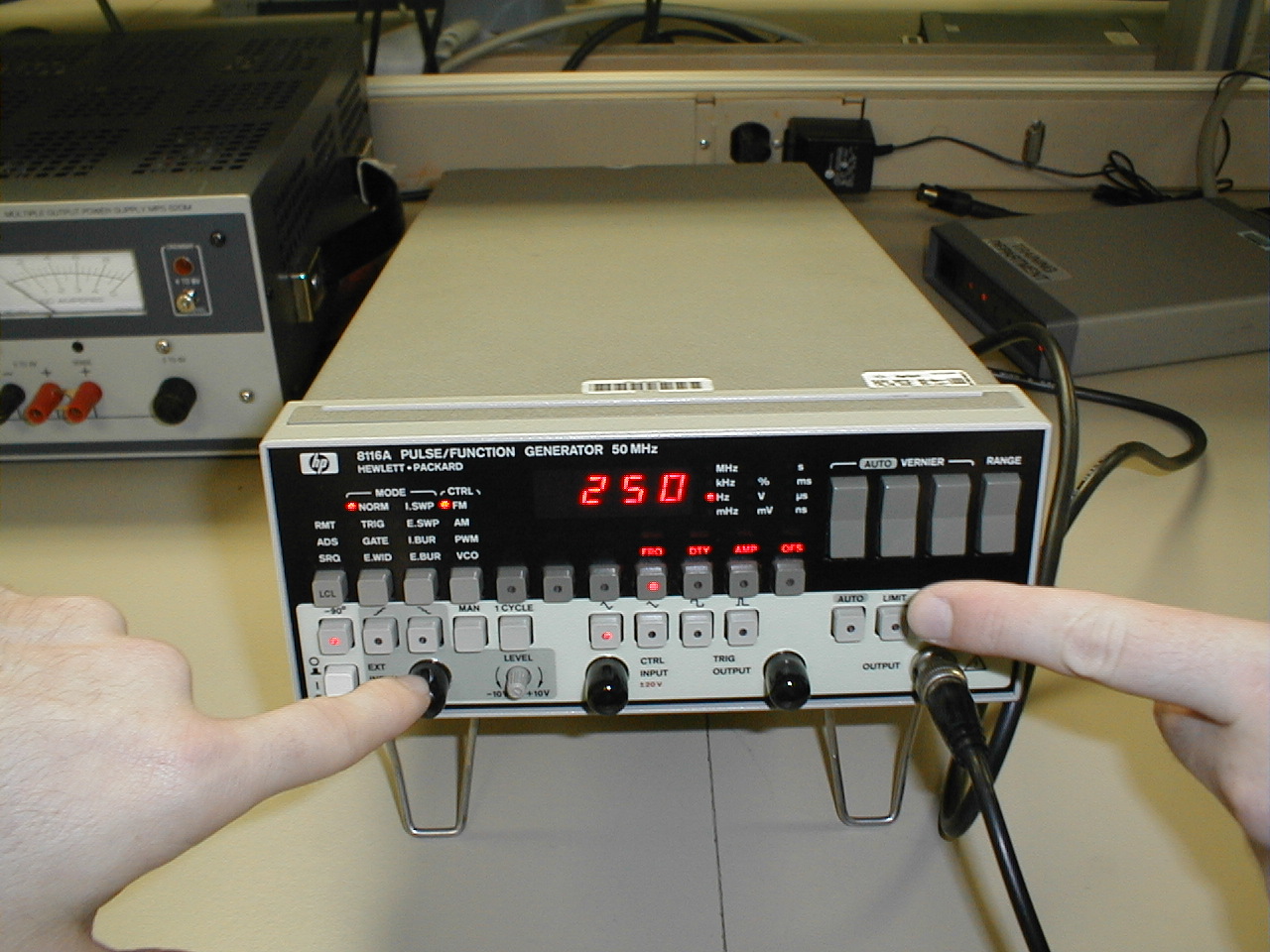
To test our circuits we used the function generator, or as Sam likes to call it, the "fun" generator.

While working on our project late into the night we found it necessary to grab a quick snack (Food Provided by Randy):

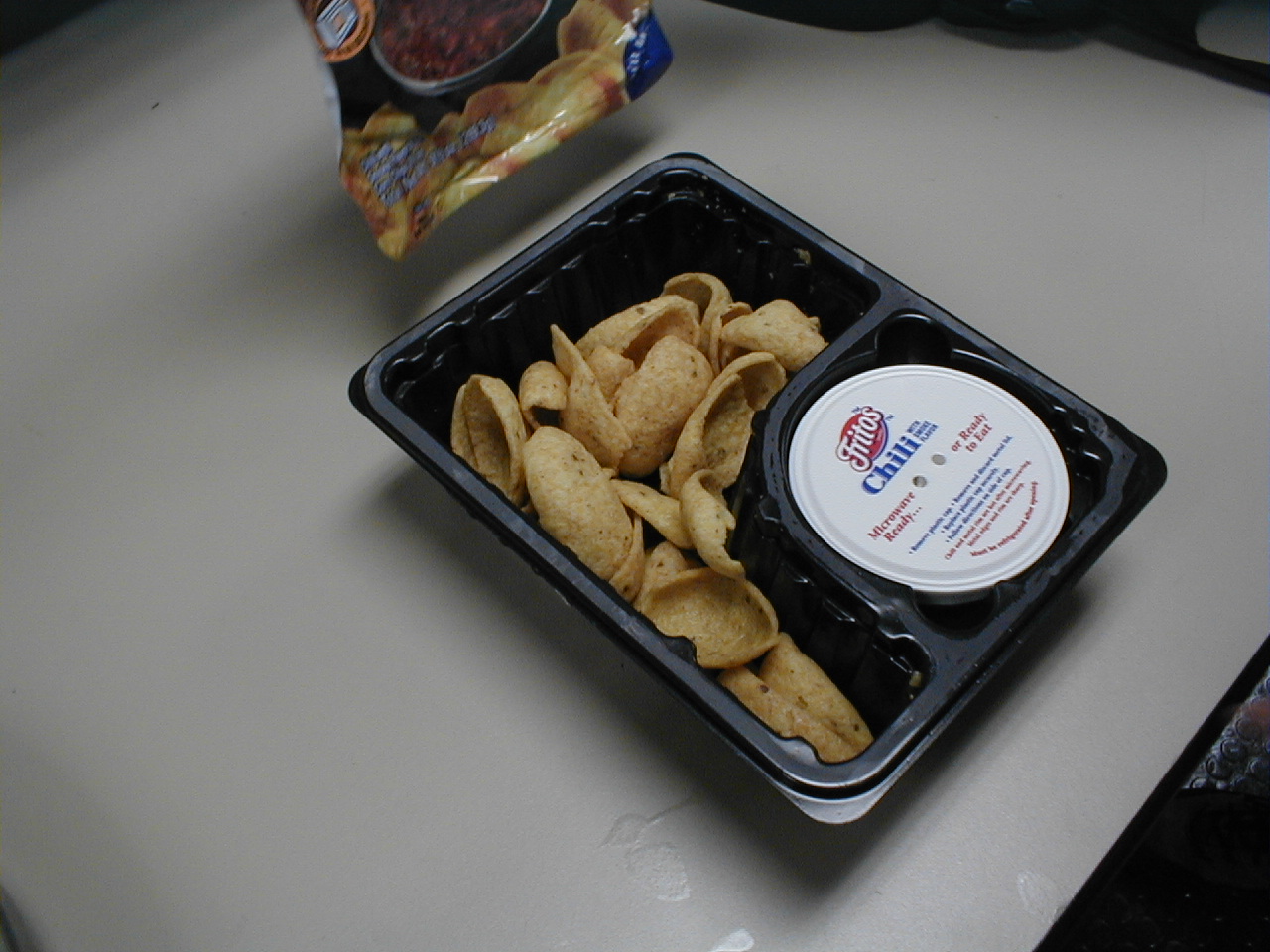
It should also be noted that Tom was still feeling that can of chili well into the following night...

As we continued our work we suddenly came upon something slightly unexpected. One of our recovered signals sounded suspiciously like one of those intercoms at a fast food drive through. We felt that this merrited a Taco Bell run (Car provided by Randy):

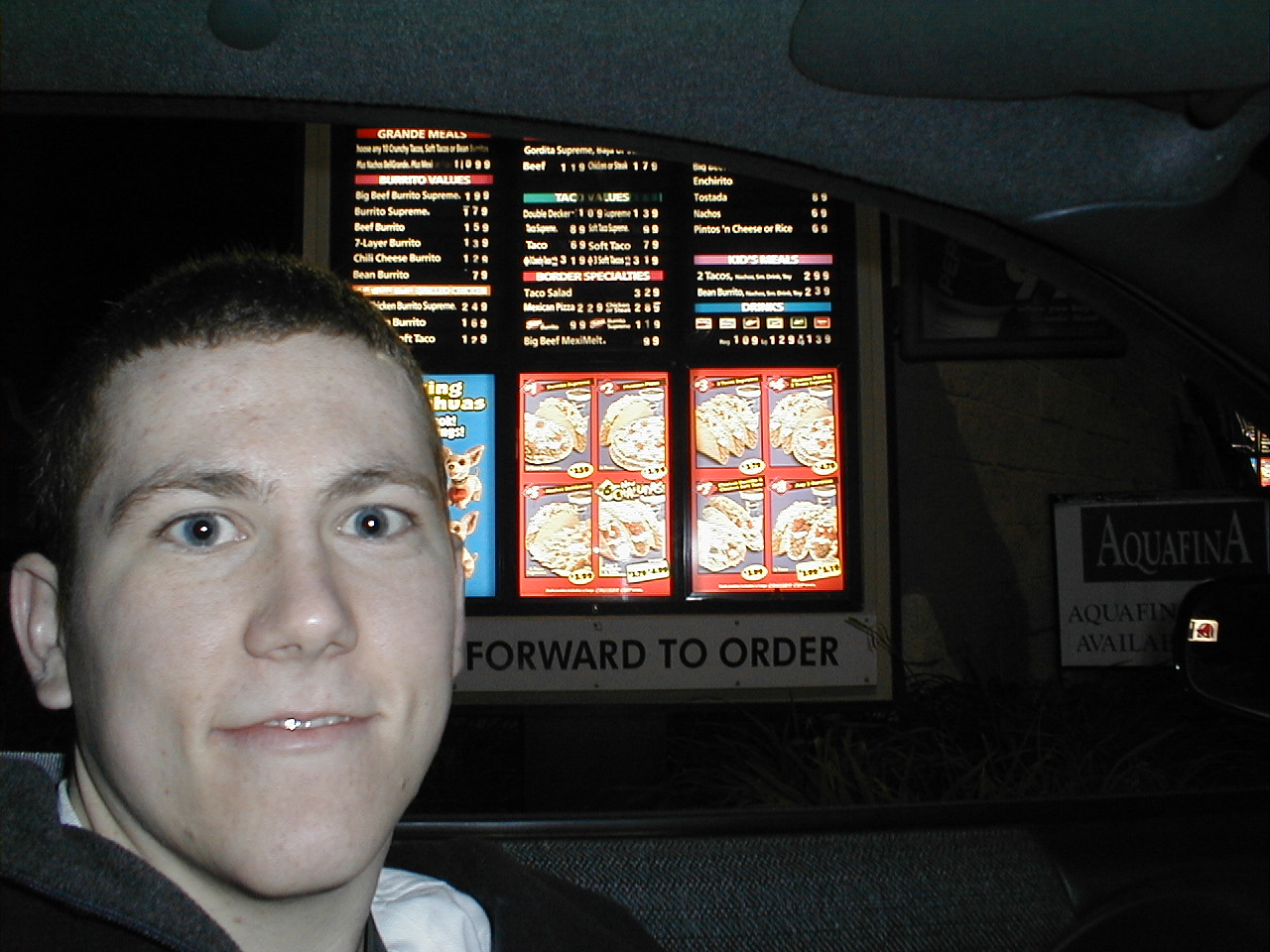
Randy loves his tacos, almost as much as he loves Trushar...

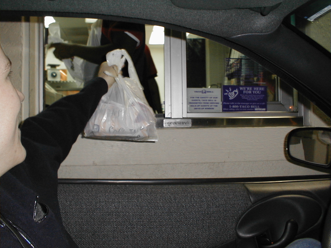
The nice man hands the food to Randy as Tom snaps a picture for posterity...

As the night wears on:

Tom has an overwhelming urge to take a nap. Maybe its the chili.

Sam tries to control his anger and pent up rage until...

He finally snaps and beats Randy with a chair