
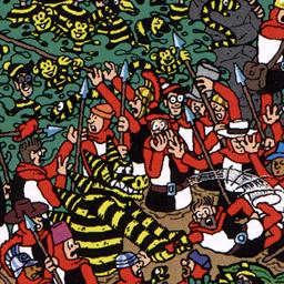
We also used smaller portions of the "Where's Waldo?" pictures as a reference because of memory constraints. Here is one reference.
When our group sat down to do this project we started with the code written by the DSP Pictomaniacs in the 1996 ELEC 431 class. We attempted to run their code on our images, but we had difficulty doing this. We decided to ignore how they had normalized their images (using correlation) and tried to normalize our images as we understood it (that is, by dividing by the norm of the matrix). Unfortunately, this did not work either. Our program was finding white spots in the picture regardless of where Waldo was. Something was clearly wrong. The solution to this problem was an energy normalization. The white areas of the picture have more energy than the darker areas, and this needed to be normalized so that the program could pick up the areas where the template and referance highly correlated. The DSP Pictomaniacs' code had accounted for all of this, but we just did not realize it. From there we were able to modify our code to deal with color and to attempt to use the Waldo head with other pictures.
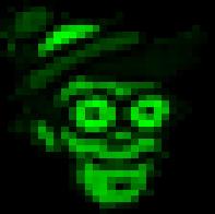
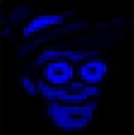
We took a picture of Waldo from one of our larger images, cropped
the image down to the size of his head and made the background behind his
head black. This became our template.
We also used smaller portions of the "Where's Waldo?" pictures as a
reference because of memory constraints. Here is one reference.
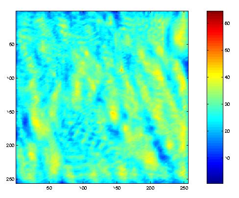
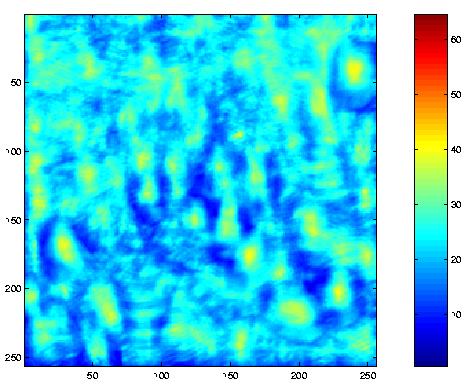
Before we convolved the two images, we normalized the energy in the
"Where's Waldo?" picture. To do the energy normalization, we convolved the
point-wise square of the matrix of the "Where's Waldo?" picture with a
matrix of ones the size of Waldo's head. Pointwise dividing the original
picture by the square root of the above matrix effectively took the local
average of the energy in the picture. We also did a standard L2
normalization of both the picture and the Waldo head, so that
the values of the inner products between the two would be between 0 and
1.
Our program completes three convolutions. This is because
in MATLAB, color is stored as an array of 3 matrices where the
values in each array represents the intensities of the colors red, green,
and blue respectively. We convolved each of the three Waldo color
matrices with the respective "Where's Waldo?" color matrices.

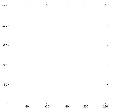
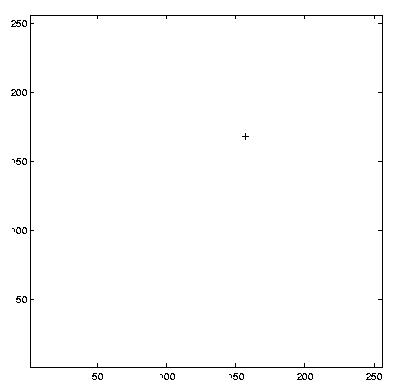
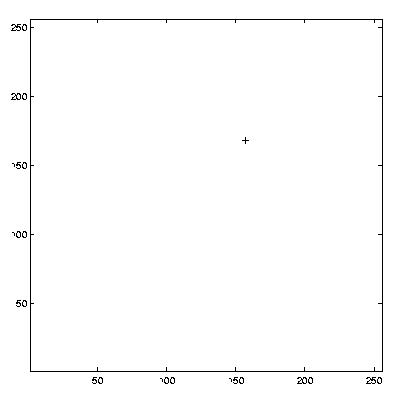
Finally, to test where Waldo was, we found the point in each of the three convolved matrices that had the highest value (look for the red dot in the left images): the Red,
 |
 |
 |
 |
 |
 |
 |
 |
% Find highest correlation of template in an image of indeterminate
size
function Waldo
clear
close all
% Scaling factor for plotting normalized correlation values over full
color
scale
scaleColor = 64;
tmpl = input('Template to find? ','s');
ref = input('Reference? ','s');
template = double(imread(tmpl));
reference = double(imread(ref));
xSize = size(reference, 1);
ySize = size(reference, 2);
for i = 1:3
% Using L2 norm to normalize intensities of reference and template.
reference(:,:,i) = reference(:,:,i) / (norm(reference(:,:,i),'fro'));
template(:,:,i) = template(:,:,i) / (norm(template(:,:,i),'fro'));
% Preflip template to conteract inherent flip in convolution
algorithm
template(:,:,i) = flipud(fliplr(template(:,:,i)));
correl(:,:,i) = conv2(reference(:,:,i),template(:,:,i),'same');
% Local average energy norm: Convolution of reference squared (to
accentuate
differences) with flat matrix of ones
flat = ones(size(template(:,:,i)));
energyNorm = (conv2(reference(:,:,i).^2, flat, 'same')).^.5;
% Normalize correlation array with local average energy norm to
discount high correlation due to more intense colors and isolate
correlation due to template pattern matching
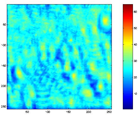
normalized(:,:,i) = correl(:,:,i) ./ energyNorm;
% Display normalized correlation array
figure
image(normalized(:,:,i) .* scaleColor);
colorbar;
axis square;
% Print position of highest correlation
[maxVec,y] = max(normalized(:,:,i));
[maxVal,x] = max(maxVec);
maxX = x
maxY = y(x)
% Display position of highest correlation
figure
plot(maxX,(ySize - maxY), '+')
axis([1 xSize 1 ySize]);
axis square;
end
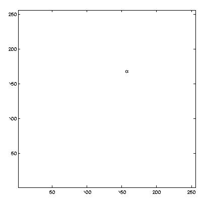
% Take composite correlation of each color(RGB) correlation matrix
composite = normalized(:,:,1) + normalized(:,:,2) + normalized(:,:,3);
% Display composite correlation
figure
image(composite .* (scaleColor / 3));
colorbar;
axis square;
% Print position of highest composite correlation
[maxVec,y] = max(composite);
[maxVal,x] = max(maxVec);
maxX = x
maxY = y(x)
% Display position of highest composite correlation
figure
plot(maxX, (ySize - maxY), 'h')
axis([1 xSize 1 ySize]);
axis square;