
Speech transcription is a large application area in which the lengthy computation time to slow down the signal would not be an obstacle. Similarly, both music lovers and musicians would benefit from the ability to slow down music. Musicians might use this function to slow down a recording of themselves and thus be able to improve their performance, or maybe to transcribe an improvisational jazz solo.
Answering machine messages constrain the listener to taking in information at the speed at which the caller recorded the message, and often this is too fast to both understand and write down. Being able to slow down a phone number or address would be a perfect application, very useful and commercially viable.
The study of foreign languages could be made easier by slowing down the speech of natives in order to better distinguish the differences between that language and the student's native tongue.
Also useful is the ability to increase the speed of speech for commercials, both television and radio. Because time is so valuable, being able to communicate more information about their product in a given amount of time would be very valuable to advertising agencies and their clients.

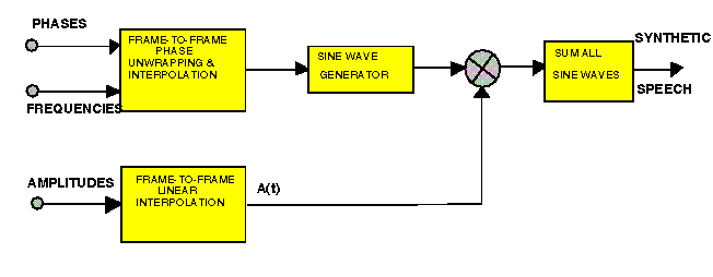
From this point the phases and frequencies are fed into a "black box" that performs frame to frame phase unwrapping and interpolation. After interpolation, the data is put into a sine wave generator. In addition, linear interpolation is performed between the amplitudes of each matched frame. From this point, the values are summed across all frames to get the synthesized speech.
The first part of the code takes the STFT of an audio signal. The file stft.m performs this function. To take the STFT on an input audio signal, the data is windowed at overlapping intervals. This overlap is measured by the distance between the peaks of consecutive windows. For each windowed segment of data, the DFT is computed, and the peaks of the DFT are picked out using peaks.m. The data returned for each window constitutes one frame, and includes the frequencies, magnitudes, and phases for the peaks of that window. The distance (in samples) between frames is the same as the distance between windows. This distance can be as small as one data point, but ideally, it is many samples. Interpolating between frames is how we slow down or speed up speech.
The next bits of code did the frequency matching between frames. The function freqmat2.m does this job. In order to match frequency peaks picked from one frame to peaks in another frame we implemented the method presented in the McAulay and Quatieri paper. The idea is to choose a matching interval that picks frequencies in the next frame that are possible matches to the frequency of interest in the current frame. In our case we iterated from the lowest to the highest frequency in a frame given as columns in a matrix returned by stft.m. We settled on an interval size of between .06 and .1 radians (i.e., delta = .03 or .05).
After picking possible matches from the next frame and taking the nearest one, the next frequency in the current frame was evaluated to see if there were any points in the next frame that were a possible match that also corresponded to the possible match that the previous frequency found. If this were the case, then we checked to see which frequency was closer to this possible match. If the current frequency were closer then a match was made. However, if the next frequency in the current frame was a closer match to the possible, then the current frequency must take a second choice. If there were no second choices available then that frequency track is said to have died and a zero is inserted. Then we do the same process for the next frequency. Notice that the next frequency has already been evaluated for possible matches so we need not do this again and we save a lot of computation time.
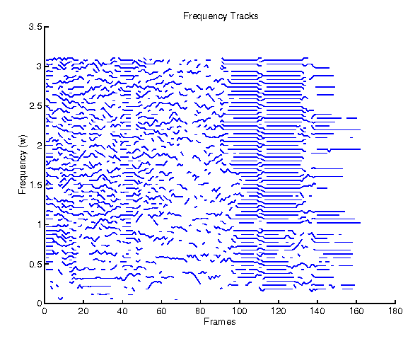
If, after going through an entire column (i.e. track), there are frequencies that have not been matched to frequencies in the next frame, they start a new track and are termed born. These new tracks are simply placed in an open area in the matrix at the corresponding frame (or row index). In this manner we were able to preserve the data an efficient manner that allowed for the easy extraction of frequency tracks. A plot of these tracks can be obtained by using trackplot.m which simply searches for tracks and plots them as lines. Figure 3 shows a sample output from this function.
The interpolation code has two parts, unwarp.m and inter.m. The idea behind phase unwrapping and interpolation is that the function connecting the information taken in each frame should be as smooth as possible. The 2-pi periodicity of phase makes the problem more difficult, but using McAulay and Quatieri's calculations, the computation was fairly straightforward.
Unwarp uses the equations given in McAulay and Quatieri to calculate the smoothing constants M, alpha, and beta for each frame. Then, the function inter.m calculates the interpolating functions for the phase and the amplitude. The phase is dependent upon the above constants as well as the current and next-frame phases and frequencies, as well as the distance in samples between the frames. The amplitude is a straight- forward linear interpolation based on the current and next-frame amplitudes.
The final signal output by the system was calculated in sumy.m. That was simply the sum of the cosine of the phases for each frame, weighted by their amplitudes. In this way, we did not have to explicitly call a function to calculate the inverse Fourier transform.
Variables we altered were the window size, the type of window, the spacing between window peaks, the interval over which we searched for a peak, and the delta that determined how selective the frequency matching was. Our best results were with a window size of 255, distance between window peaks of 1, peak searching interval was 5, a Hamming window, and a frequency matching delta of .03. With these parameters the character of the person speaking was intelligible, as was the general structure of the word, but a control person asked to identify the word (not knowing the test word beforehand) would likely have been unable to identify the word. Thus, our largest problem was distortion.
It was also a bit disappointing that we had to set the distance between windows to 1 in order to get intelligble synthesized speech from our model. Since we set this value to one, and speding and slowing of speech is done by interpolating between frames (i.e. adding or reducing samples), we clearly cannot speed up speed, since we can't reduce the samples any more without losing information.
Choosing a window size of 255 gives a broad spectrum and helps select accurate frequencies to characterize the signal. However, such a large window means we do not equally weight the first and last samples of the signal. A fix would be to zero pad the signal so that all of the samples were given equal weight by the windowing mechanism.
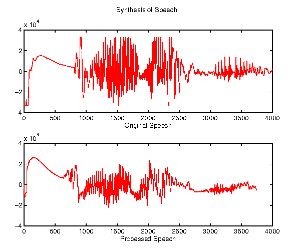
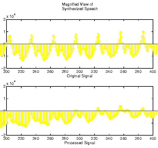
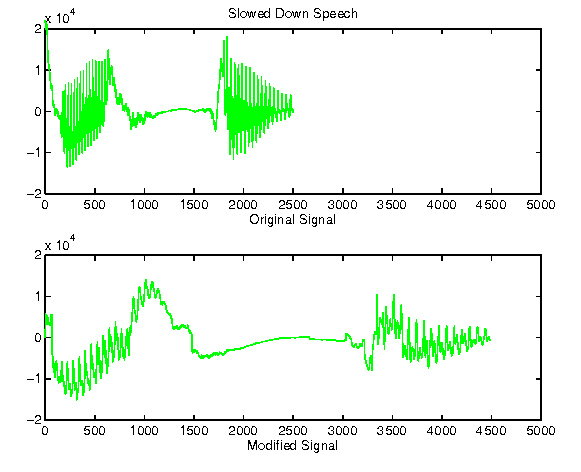
Figure 4 shows an example of synthesized speech. You can clearly see from the picture tat the waveform itself is an excellent match. However, due to some distortion, higher frequencies are lost (i.e. the peaks aren't as sharp).
Improving computational time is a non-trivial problem. The system can be seen as a series of algorithms, and due to the nature of the data and the processing necessary, the algorithms are all on the order of N2. Without creating completely new algorithms, it seems theoretically impossible to lower their order and thus computation time improvements must come from lowering how much data we are processing in any one stage. Lowering how much data, i.e. information, could make distortion worse (because we would be working with less information) or it could remain the same or even improve if other changes were made. One such improvement might be to use a smaller delta to ensure a tighter match within a track, and using less tracks to reduce the computational load.
Using a DSP chip would reduce the problem of computation time significantly. The algorithms, bulky though they are in Matlab, would reduce in length dramatically and the process could approach real-time for shorter signals.
Overall, we were fairly pleased with our project. Although we produced no spectacular results, we felt we learned a lot of about speech processing and now have a full appreciation for the difficulty of the task.