Linear Predictive Speech Coding
Introduction
For low bit rates, directly encoding a speech waveform is not a viable
option. The waveform is not very localized in frequency, and thus
cannot be coded efficiently. We have to turn to a model based
approach.
LPC Coding
LPC consists of the following steps
- Pre-emphasis Filtering
- Data Windowing
- AR Parameter Estimation
- Pitch Period and Gain Estimation
- Quantization
- Decoding and Frame Interpolation
Pre-emphasis Filtering
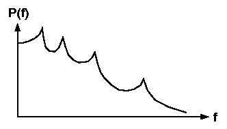
When we speak, the speech signal experiences some spectral roll off due
to the radiation effects of the sound from the mouth (see the Figure
below). As a result, the majority of the spectral energy is concentrated in the lower frequencies.
However, the information in the high frequencies is just as important
to us understanding the speech as the low frequencies; we would like
our model to treat all frequencies equally. To have our model give
equal weight to each, we need to apply a high-pass filter to the original signal.
This is done with a one zero filter, called the pre-emphasis filter.
The filter has the form:
where a is generally a value around 0.9. Most standards use a = 15/16
= .9375. Of course, when we decode the speech, the last thing we do
to each frame is to pass it through a de-emphasis filter to undo this effect.
Data Windowing
We will assume that a speech signal is a stationary AR process over
a short amount of time. However, to avoid discontinuities in the model,
we will use overlapping data frames. As the frame size gets larger
and larger, our bit rate gets lower and lower, but of course our
assumption of the process being stationary over a frame becomes more
and more precarious. For the LPC coder implemented in this project,
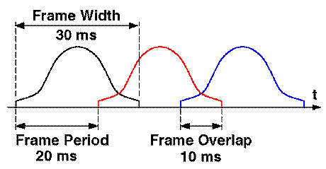
we used a frame size of 240 samples. Since we used speech signals
recorded at 8k samples/sec, this amounts a frame width of 30 ms. We also used a
frame overlap of 10 ms (1/3).
Sometimes it is desirable to window the data to lower the variance of
the autocorrelation matrix estimate. The standard bias-variance
trade-offs for the AR estimate (autocorrelation estimate) occur for
different data windows. In this project we used a Hamming window, as shown in the figure below.