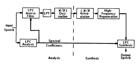
Rather than parameterize the residual signal as white noise or an impulse train as in LPC-10, RELP encodes the actual residual signal. This requires a higher bit rate, but does a better job of capturing the true characteristics of the residual signal. This, in turn, yields a better reconstruction of the data signal.

Golden Steps to RELP
First, a tenth order AR model is constructed by solving the Yule-Walker equations with the Levinson algorithm. This is the same model that is employed in the LPC-10 algorithm, using a biased ACF estimate.
Next, The AR model is used to construct a forward error prediction filter. The forward error prediction filter computes the residual between the actual data and the predictions.
In order to get a significant reduction in bit rate over coding the original signal, the residual needs to be downsampled. This requires an anti-aliasing filter. Our experiments used a Cheby I filter with normalized cutoff frequency of .25 and .05 dB ripple in the passband, allowing us to downsample by a factor of four.
We downsample by a factor of four.
We quantize the downsampled residual using a Lloyd-Max quantizer. One, two, four, or eight bits per sample are allowed in our program.
Once the signal is received, it is first upsampled in order to get the proper length. For our experiments, this is a factor of four.
Next, we need to regenerate the high frequency part of the spectrum. Adding copies of the baseband to the higher frequency bands is a reasonable approximation if enough of the baseband was kept by the anti-aliasing filter since much of the high frequency components are related to the baseband by harmonics. We actually get this for free when we upsample since the copies get compressed into the spectrum. This would not be the case, however, if the data was complex. Real data has a symmetric frequency representation so that when the copies are added to the higher frequency ranges the spectrum will be continuous. Had we been dealing with complex data, the spectrum would not have necessarily been continuous by just adding copies in the higher frequency ranges. A technique called spectral folding is used in this case to make the spectrum continuous. Every second copy that is added to the higher frequency ranges is flipped so that the entire spectrum is continuous. This enhances the performance of the reconstruction when dealing with complex data.
Finally, the reconstructed residual is used as the driving signal into the AR model to get the estimate of the original signal.
|
| BACK | NEXT |
|