Time-Frequency Analysis

Introduction

The purpose of this project is to code and experiment with four of the primary time-frequency analysis techniques. The four techniques are the short time Fourier transform (STFT.m), the discrete wavelet (Haar) transform (DWT2.m), the continuous wavelet (Morlet) transform (CWVT.m), and the pseudo-Wigner distribution (PWD.m). Each of these transforms were coded in MATLAB and tested on a chirp signal (i.e., an increasing frequency as time increases). After successfully implementing the transforms, the code was used to investigate a real world signal. In our case, the closing price of Micron Technology stock over a decade was used.

Real World Data

The analysis data (mu.m) is the closing stock price for Micron Technology. It has long been held that the DRAM memory business has a cyclic revenue stream. Several companies produce DRAMs, but this is usually only one of many sectors within any specific company. Financial figures for any one sector of a company are not generally available. Micron (ticker symbol: MU) has both memory and personal computer sales, but their foundation rests on the semiconductor side. This makes their stock the best indicator of the memory business outside of proprietary financial data.

The data is a bi-monthly sampling of the closing price roughly over a ten year period (256 sample points). The file (mu.m) contains the split adjusted price of the stock. Comments in the file show the date of the closing price and the split adjustment. The file (mu1.m) contains the same data as mu.m, but is not split adjusted. The last file, (mu2.m), is the same data as mu1.m, but contains a dollar cost adjustment equal to a 3% annual percentage rate compounded monthly (0.25% / month).

Since we are interested in the cycle of the stock, and not the growth factor, mu2.m data was used. Furthermore, the log (base exp) was applied to flatten the data, and finally, the mean was subtracted. This gives us a zero mean signal with a dollar cost adjustment to the closing price of the stock. The original mu.m and adjusted signal (log(mu2.m)-mean(mu2.m)) are shown at the top of Fig. 2.

Short Time Fourier Transform

The short time Fourier transform (STFT) function is simply the Fourier transform operating on a small section of the data. After the transform is complete on one section of the data, the next selection is transformed, and the output "stacked" next to the previous transform output. This process allows the type of window, window length, and zero padding within the FFT to be adjusted. The window type for our code include rectangular, Hamming, Hanning, and Blackman-Tukey. The results from the chirp signal are shown in Fig. 1. The real world data results are shown in Fig. 2. Only our "best" results are displayed in Fig. 2.

Figure 1.   Short time Fourier transform of chirp.m

As seen in the last frame of Fig. 2, two markers have been added to indicate strong frequency peaks. The lower frequency is approximately equal to a period of 4.6 years. The higher frequency marker corresponds to approximately 1.7 years, but has substantially less energy. Overall, the data appears to have several harmonic frequencies that are time varying. Just by looking at the time based data in the second from the top frame, one can envision a sinusoid that goes negative at time zero, peaks at 130, then goes negative again. This implies a cycle of about 5 years, which corresponds with our results.

Figure 2.   Short time Fourier transform of the real world data

Discrete Wavelet (Haar) Transform

The discrete wavelet Haar transform uses a different basis than the STFT. The STFT uses complex sinusoids, with increasing frequency, which are shaped by the window function. Wavelet transforms, on the other hand, maintain the same number of oscillations within the window, but compress or dilate the window to adjust the frequency. It has other properties such as the function must always be bandpass. A wide variety of basis functions are available. We used the most basic: the Haar wavelet. The results from the chirp signal analysis are shown in Fig. 3 with varying degrees of resolution in frequency (~ scales).

Figure 3.   Discrete wavelet (Haar) transform of chirp.m

The results from the DWT support the STFT data, but more coarsely. The final frame in Fig. 4 shows several spikes at 0.02 which is in between the markers in the STFT results. One interesting observation, which shows the value of different analysis techniques, is the high spike across multiple frequencies in Fig. 4 at approximately 140 (70 months). This is due to the large downward step taken by the stock at that point. Similar results can be show with the STFT, but not with the same window length. The DWT captured in one plot, both the smooth and spiky trends in the data.

Figure 4.   Discrete wavelet (Haar) transform the real world data

Continuous Wavelet Transform

The Continuous Wavelet Transform (CWT) has much in common with the Short Time Fourier Transform (STFT). The big difference is that the windowing function shifts frequency by scaling rather than modulating . The equation for the CWT is as follows:

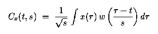
where x is the signal, w is the wavelet function, and s is the scale variable (dimensionless). The wavelet function is analogous to the windowing function of the STFT and scale is analogous to frequency. The wavelet function must be square integrable and be bandpass (have no energy at zero frequency). We used a real Morlet Wavelet, which holds for the above properties and has the following form:

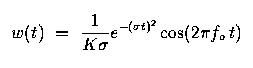
where sigma is the approximate bandwidth and fo is the center frequency. The following figure shows examples of the Morlet wavelet function at three different scales, along with the corresponding frequency domain information.

Figure 5.   Morlet wavelet at different scales

Note that frequency resolution is proportional to bandwidth, so it will decrease at higher frequencies and increase at lower frequencies. Accordingly, we get higher time resolution at higher frequencies and lower time resolution at lower frequencies. This is not the case for the STFT, where the frequency resolution is the same over all frequencies. Finally, we implement the CWT by sampling at t = n/s. The following picture depicts our implementation of the CWT over four scales using chirp.m as our input signal.

Figure 6.   Continuous wavelet transform of a linear chirp signal

Note that at lower scales we have better time resolution, as we would expect. We can also see the chirp has a more even frequency spectrum as our time resolution gets worse (frequency improves). This corresponds to a what we might see with a Fourier Transform of a chirp, which has perfect frequency resolution and no time resolution (so we just see an even spread of energy at most frequencies). We also see the linear time versus frequency characteristic of a chirp signal.

Next we tested the CWT on real world data. "mu2.m" was used as our signal, with the adjustments to this signal explained in the "Real World Data" section above. The following figure shows the CWT of this input data.

Figure 7.   Continuous wavelet transform of real world data

We see that at the lowest scale we have a pretty smooth spectrum. This corresponds to poor frequency resolution and the limit amount of high frequency components in the data. We can see brighter peaks around t = 160 and t = 250, just like our data. The peaks at low t correspond to the wrapping we did to periodize our data. We can see that as our scale gets bigger (better frequency resolution), we have some localization of energy carrying over scales. This tells us that we have higher frequency components at these times.

Pseudo-Wigner Distribution

The MATLAB function PWD.m calculates the pseudo-Wigner distribution. The function was tested with the chirp signal in chirp.m and the result is shown in Fig. 8.

Figure 8.   Pseudo-Wigner distribution of a linear chirp signal

As expected, the time-frequency representation clearly shows a linearly increasing frequency characteristic with increasing time. The Wigner distribution gives the best time-frequency resolution.

We obtained the Wigner distribution of the real world data "mu2.m" to analyze its time-frequency characteristics. The result is shown in Fig. 9. Most of the variations are slow (low frequency) with period greater than a year. The distribution shows a low frequency component at a normalized frequency of around 0.007 (approximately a period of 5.9 years) for most of the time duration. This is expected from the earlier results using the STFT.

Figure 9.   Pseudo-Wigner distribution of the real world data

Conclusions