Navigation:
Introduction/Overview
Process
Application
Synthetic vs. Natural
Comparison
Conclusions
MATLAB Code
Extras
Application
As explained in the overview, EMD is most useful (and as we will see later, perhaps only useful) for non-linear, non-stationary signals, and natural signals. As an example of this, we have applied the EMD to several signals, two of which are the raw data from electrocardiograms that we found on the web. The horizontal axis represents sample number, as sampling rate was not available for both.
Note: If using a new browser that typically fits pictures to windows, make sure to maximize any full size signals you decide to view or they may appear distorted or fuzzy.
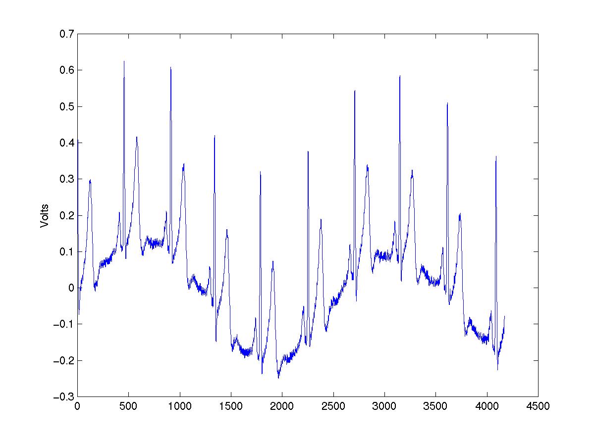 ecg.mat
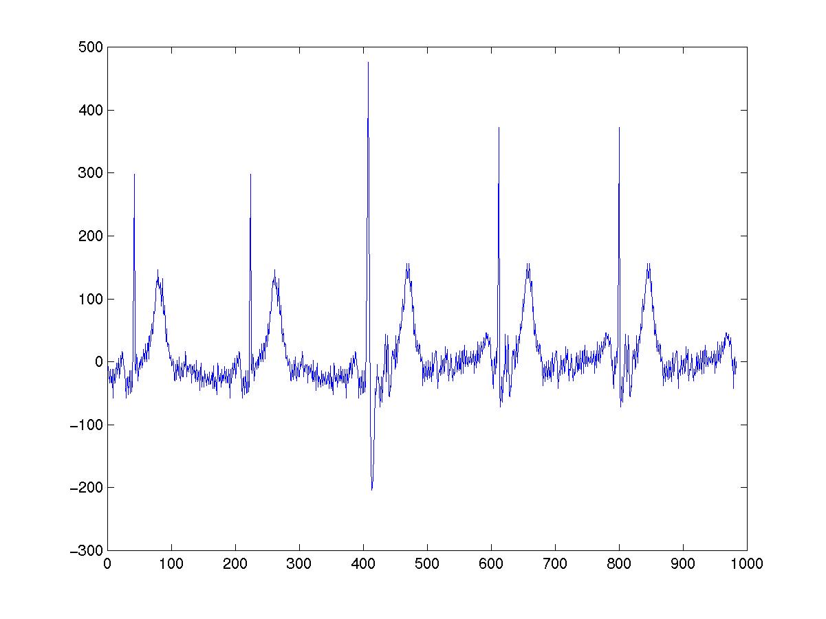 ekg.mat
The following are the results when the EMD is applied to each signal; the axes are the same as the original signal plots:
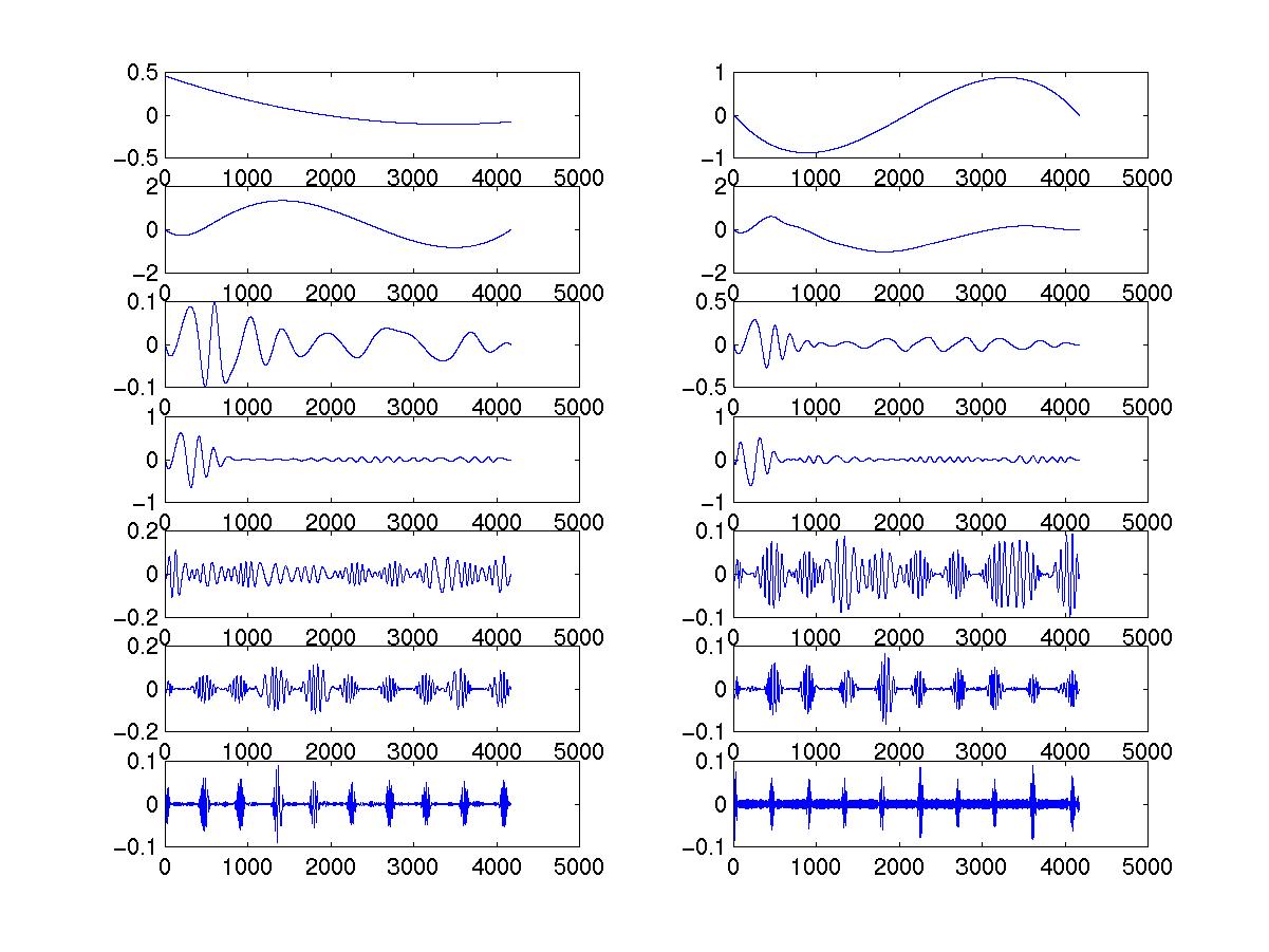 ecg.mat
Plots run from c14 on the upper left to c1 on the lower right.
 ekg.mat
Plots run opposite; from c1 to c14.
Each IMF represents a different part of the signal, giving a fairly good breakdown of different causation parts of the total composite heartbeat. While the wave in ecg.mat (of which we still cannot determine a cause) causes the EMD some problems, the signal ekg.mat was broken down fairly efficiently, especially in IMF c3, where each heartbeat has been identified as a single entity amidst the other lesser parts that together compose a single beat.