COMP 130 Elements of Algorithms and Computation
Spring 2012

General Coupled System

Note:  COMP 130 students are NOT required to know how to do the partial differential equations techniques used in the following derivations!   The important issue here is to see the form of the mathematical results and to be able to use those results.   The derivations are presented simply for completeness and rigor.

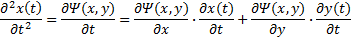
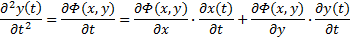
Consider the following generalized coupled differential equation involving x and y, where both are functions of time and are related by two first-order coupling functions, 𝜳 and 𝜱:

These first-order equations are of the type that were used to create the our existing first-order Lotka-Volterra algorithm:  

(The t₀ subscript refers to the value of that derivative or function evaluated at time t₀.)  

But to refine that approximation, we need to calculate the second derivatives with respect to time using partial differentiation:

Substituting our original equations back in:

The second-order Taylor series expansion of x(t) and y(t) around time t₀ is thus:

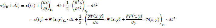
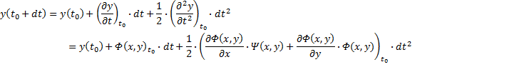
Notice that the symmetry in  𝜳 and 𝜱 that was present in our original couple derivatives above is reflected in the second-order Taylor series expansion we have here.

Also note that there are really only 8 distinct quantities represented in the above result:

• (2) The current values of x and y (i.e. evaluated at t₀)
• (2) The current values of  𝜳 and 𝜱 (i.e. evaluated at t₀)
• (4) The current values of the derivatives of  of  𝜳 and 𝜱 with respect x and y, evaluated at t₀.

Thus, to calculate the next time step in the  x and y curves to second-order accuracy, since we are given the current values of x and y, to calculate the next values, we need only calculate at most 6 distinct quantities.

 

2^nd Order Lotka-Volterra Model

In the Lotka-Volterra equation for predator-prey modeling, the coupling equations are

Here, x(t) is the prey population and y(t) is the predator population and thus the variables are defined as:

 

In order to perform the calculation of the 2^nd order Taylor series expansion, the four partials must be calculated:

Armed with the 4 calculations above plus the 2 calculations for 𝜳 and 𝜱, which are the first-order time derivatives for the prey and predator populations respectively, one can now construct the 2^nd order Taylor series results for the hare and lynx populations as per the equations from the last section above.

The next level?

Consider thes notions: 

• If the curve we are trying to approximate is a straight line, the a 2nd order solution is not advantageous because the second derivative is always zero.  
• The second derivative, or more generally, the next higher derivative is always much more of a pain to compute.
• But if the step size is small enough, one can always reduce the error to an arbitrarily small level.
• Uniformily small steps greatly increases the number of calculations required.

But why don't we just use small step sizes only where we need it?    Crudely, if we are doing a first-order approximation, the larger the second derivative, the smaller the step size.

These sort techniques are called "adaptive step size" methods.   Examples of adaptive step differential equation solvers:

• Adaptive Runge–Kutta methods
• Runge-Kutta-Fehlberg method

Unfortunately they are way beyond the scope of this class.   Take a CAAM class (e.g. CAAM 353) to learn more.

More Effects?

Let's continue on and investigate adding some new effects to the Lotka-Volterra model, such as a limited environmental carrying capacity, which means that animals could starve to death if their populations get too high:   Prey Starvation in Lotka-Volterra