COMP 130 Elements of Algorithms and Computation
Spring 2012

Prey Starvation in General

Note:  COMP 130 students are NOT required to know how to do the partial differential equations techniques used in the following derivations!   The important issue here is to see the form of the mathematical results and to be able to use those results.   The derivations are presented simply for completeness and rigor.

These notes are supplementary to the class notes on Prey Starvation in the Lotka-Volterra model.

In general, the effect of  exceeding the "carrying capacity" for the prey is that the prey's population rate (w.r.t to time) gains an additional negative term, S_x(x) below, when the prey population exceeds a certain threshold, what we will call the "cutoff" value, x_cut below.    Above that value, the prey population begins to be affected by losses due to starvation.  Below the cutoff, nothing has changed from our previous models.    The first-order term of the Taylor expansion of our system is thus modified by the addition of a single function call:

For generality, the negative sign of the starvation effect is encapsulated in the S_x(x) function.    Also, one could simply say that the starvation term,  S_x(x), always exists in the formula, it's value is simply zero below the cutoff.    In fact, this is the easier way to represent the equation, computationally.

To create a model of the starvation effect, we need to consider a couple of phenomena that our model should reproduce:

1. Below the cutoff population, the effect is zero.
2. Above the cutoff, the effect is starting from zero and monotonically increasing.    That is, there should be any overly abrupt transition to the onset of the effect and that the effect gets more and more pronounced as the population climbs.

To make our lives easier, we will define a population, x_max, where the starvation effect defined to be exactly equal to the population at that point,  that is, S_x(x_max) = -x_max.   This means that at x_max, the starvation rate is 100% per year.    By expressing the starvation effects in terms of  x_cut and x_max , the magnitude of the starvation effect can be controlled by setting more tangible values than abstract coefficients in a mathematical formula.

There are many ways to model the starvation effect.   Here we will look at a linear model and a quadratic model as two possibilities.   Note that the plot below is of the negative of the starvation effect term.

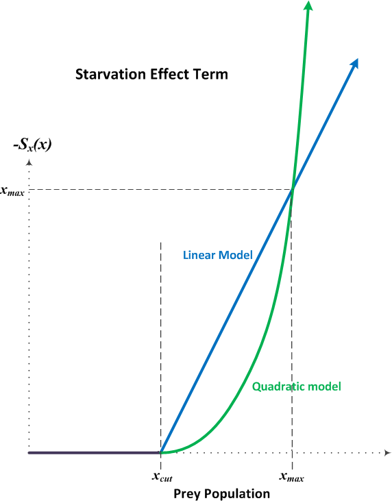
IMPORTANT: Remember that the starvation effect term only affects the system for populations above the cutoff population, x_cut!  Below the cutoff, the term does not appear at all in the calculations and everything is as it was in our previous models.   Note that this statement is consistent with saying that S_x(x)=0 below the cutoff.

 

Linear Model

A linear model is the simplest model that one can make that matches the above criteria.    Here, the starvation effect grows at a rate exactly proportional to the population.    One could argue about its realism, but often times, as a first cut in modeling, one simply wants to see whether or not a model with the correct basic characteristics produces viable results at all.   If that can be shown, then one can proceed towards creating more detailed and more accurate models.

In the linear model, the starvation effect comes on abruptly above the cutoff point, rising in a straight line.   This can be represented as a simple linear equation in the prey population:

The effect on the second-order approximation for the Taylor expansion of the prey population is only in one of the partial differential calculations, where it simply subtracts a constant value, which is just dS_x(x)/dx:

Notice how the value of this term abruptly changes from just below the cutoff, where there's no constant term on the end, to just above the cutoff where that constant value at the end suddenly appears.

To isolate the starvation effect from the rest of the model, this additive contribution to this one partial derivative calculation should be encapsulated in a second starvation function (the derivative of the first with respect to the prey population) that, similarly to the linear term above, that is added to the original partial derivative calculation.

Nit-picking technical note:   Since the full second order term of the Taylor expansion includes 𝜳 as well as the partial derivative discussed above, contributions to the full second order Taylor expansion term  from the starvation model does technically come from both the partial derivative as discussed above, as well as from  𝜳 because  𝜳 does contain a starvation effect contribution (see the first order term discussion above).   Luckily, because of our careful functional decomposition, the contribution from 𝜳 is automatically handled and we don't have to worry about it at all.   Our functional decomposition shows us that the starvation effects that may be in  𝜳 are automatically included in the full second order Taylor expansion term without any additional work because  𝜳 was already calculated for use in the first order Taylor expansion term and we can simply use that value, whatever it may be, in our second order term calculation.   In our code, the only place that starvation appears expressly for the second order calculations, is in the one partial derivative.     

 

Quadratic Model

A simple quadratic model has the basic required characteristics, but has the additional feature that the transition into the starvation effect from below the cutoff to above it, is very smooth.    Specifically, the slope of the effect is zero (flat line) below the cutoff and it is also zero just at (and minutely above) the cutoff point.     The effect gets stronger and stronger as the population increases above the cutoff, much faster than the linear model.   This is consistent with the reasonable notion that starvation effects would grow faster than than the population above a certain point.

Note that for populations less than  x_max, the quadratic model actually predicts a smaller effect than the linear model.   Above x_max, however, the quadratic model predicts a much stronger effect.   This can be easily represented using a quadratic equation:

The effect on the second-order approximation for the Taylor expansion of the prey population is only in one of the partial differential calculations, where it simply subtracts a value linear in the prey population, which is just dS_x(x)/dx again:

Notice how the value of this term does not change at all as one goes from just below the cutoff point, where there is no extra linear term, to just above the cutoff, where the linear term exists but its value is essentially zero.

As in the linear model, this contribution to this one partial derivative should be encapsulated in a function, derivative of  that is simply an additive term to the original formula.

The nit-picking technical note discussed at the end of the linear model applies to the quadratic model as well.

Implementation

Because of how we carefully decoupled the various components of our basic Lotka-Volterra model, adding in the starvation effects is very easy.   In fact, the code is only impacted in two places (2 functions), whether we use the linear or quadratic starvation model:

1. The calculation of  of  𝜳:   The original code for this function is modified by an additive term that is the call to the starvation function S_x(x). 

2. The calculation of  the derivative of  𝜳 with respect to the hare population:   The original code for this function is modified by an additive term that is the call to a function that is the derivative of the starvation function S_x(x) with respect to the hare population. 

In S_x(x) and its derivative, an if-else clause is all that is needed to either include or not include the starvation effect term based on whether the hare population is above or below the cutoff value.   Likewise, an if-else clause is all that is needed to select between the linear and quadratic models.

Notice how the decoupling we achieved by decomposing the predator-prey algorithm into small, minimally-connected pieces helped to isolate the changes due to adding in the starvation effects to just a few locations!