![[Rice University]](http://www.staff.rice.edu/images/staff/branding/shield.jpg)
Understanding Our Predator-Prey Algorithm & Code
Let's first consider why we, as ecologists, would have written an algorithm and code to model predator-prey populations.
We could want to predict the future, e.g., to see whether an endangered species breeding program is likely to be successful, or could want to explain the past. In the latter case, we presumably have data that we want to compare to the model's results.
We could be creating and testing our own model, or using an existing model. In the former case, a primary goal is to understand and possibly improve the model itself. In the latter case, we likely understand the model, but want to see how well it matches existing data.
Is Our Implementation Correct?
To err is human, and making mistakes in an algorithm or code is very common. If we run it and obtain population results, how do we know if these numbers are correct? In some scenarios, we can compare to other implementations or existing data, but that is only a partial answer.
Data can be inaccurate
The lynx and hare population data depicted above is widely used because its essentially the longest-term population study in existence. The graph comes from Odum's Fundamentals of Ecology, which cites MacLulich's Fluctuations in the numbers of varying hare. The data itself comes from Hudson's Bay Company's records of pelts turned in for trading. Data could be skewed by disease outbreaks among the Native Americans doing much of the trapping during these years. Some authors caution that the data is actually a composition of several time series, with some lynx data missing, and should not be analyzed as a whole.
Models are inaccurate
Any model is an approximation of the complexities of reality. For example, the Lotka-Volterra model we are using ignores factors such as prey deaths from old age (if they don't get eaten), overgrazing (if there are too many), weather (essentially random), and other predators.
A brand-new model has yet unknown inaccuracies, and improving the model is likely to be one of the goals.
Implementations are inaccurate
At a minimum, an implementation is almost guaranteed to introduce some numerical inaccuracy. In the in-class example, we rounded populations at each step to integers. Using floating-point numbers only reduces the inaccuracy, as they still round numbers like 2 ⅓ to something like 2.3333333333333.
Larger inaccuracies resulting from algorithmic choices are also possible, and there is a whole field of measuring and reducing these. (See CAAM 353, Computational Numeric Analysis.)
Of course, an implementation could simply be wrong. Making mistakes, such as typing a formula incorrectly, is very easy to do, and hard to catch.
Exercises & Discussion
Download and save the code presented in class.
We could compare this code's results to existing implementations
(such as
this one,
where its “efficiency” is our
conversion/predation).
But, it is actually fairly easy to find a set of input values for
populations() that produces undesirable values.
Work with your neighbors in class and
- Describe what population behavior would clearly be wrong.
- Find inputs that result in that behavior.
Similarly, find inputs that produce the behaviors asked for on Assignment 1.
Understanding the Main Cause of our Code's Inaccuracy
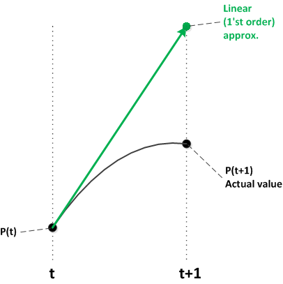
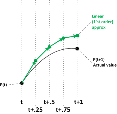
While it might not be obvious from the original problem wording, the population changes are meant to be smooth curves. Instead, we interpreted them as annual changes, which essentially means that we have a straight line from one year's population to the next. This is an inaccurate approximation.
As illustrated by the above diagrams, a simple way to make this kind of approximation more accurate is to use smaller time intervals. Each line segment uses the curve's current slope. As the intervals get smaller and smaller, the resulting segments more closely approximate the curve.
Using more technical language, the Lotka-Volterra equations are continuous differential equations:
∂pred ⁄ ∂t = pred · (conversion · prey - death)
Δpred ⁄ Δt = pred · (conversion · prey - death)
Improving the Code's Accuracy
Generalize the code so that you can control the time interval size. We'll gently guide you through the changes, but you need to figure out the exact syntax.
As always, let's first consider what our modified algorithm and code is supposed to do. Overall, our purpose hasn't changed much. We still want to compute a series of populations, given the various inputs.
We need to change the inputs slightly. Since we can vary the time interval, we need to provide that as an input. More specifically, we'll provide it as a number of steps per year. Thus, the value 365 indicates updating the population data daily.
We also need to change the outputs slightly. We still want to produce
a series (list) of prey populations and a seires (list) of predator
populations. But, observe one detail in the current code.
Consider if years=5.
Currently, the generated lists represent populations at times
0, 1, 2, 3, and 4. Those times are not returned by populations,
and it is just an implicit assumption. In fact, we later generate that list
using the code range(len(prey)) as an
input to plotPopulations.
Rather than those times being just implicitly known, it would be better
if they were explicit. So, populations should return a
list of the times whose populations are also returned.
So, now on to the code changes. Ask your neighbors in class or the course staff if you have any questions.
- Copy the provided code file, creating a new version that you'll edit.
- Add another parameter that represents how many steps per year to make. Update the documentation string to reflect the modifications in what the function will do.
-
Edit the
forstatement. Instead of iteratingyearstimes, how many times do we now need to iterate? - Edit the formulas in the loop body. Each change in population needs to be divided by the number of time steps per year. Equivalently, but mathematically more common, the change in population needs to be multiplied by the length of the time (the reciprocal of the number of steps per year).
-
Build a list of times.
- Initialize it before the loop. Assume we start at time zero.
- Add each new time value inside the loop.
- Add it to the values being returned.
-
Change the call to
populations.- Provide a value for the additional input.
- Assign the additional output to a variable.
-
Change the call to
plotPopulationsby using the list of times returned bypopulations.
Test and debug.
Experimenting with the Improved Code
As we increase the number of steps per year, or equivalently, decrease the time intervals, the resulting population curves should converge upon the desired continuous model results. Experimentally, we would like to verify this, as well as determine how small a time interval is good enough.
- Choose a set of rates (growth, predation, conversion, and death) that you'll keep constant in the following steps. It's best if you choose rates that are moderate — populations aren't neither too constant nor too rapidly changing.
-
Run
populationswith a variety of steps values, from one and higher. Plot the data, and compare the resulting plots.- As the number of steps get higher, do the resulting curves converge? I.e., do they successively look like smoother versions of the same curve?
- Above what number of steps do the resulting curves not change perceptibly?
- Repeat with another set of rates. Do your answers change?
As a challenge, how would you write algorithms and code to answer the previous questions, rather than relying upon visual inspection of the plotted curves?
Where could we go from here?
We have only scratched the surface of algorithmic issues that affect the implementation's numeric accuracy. We'll point out two directions that we could pursue from here.
When the population curves are already pretty straight, then decreasing the time interval is less important. Conversely, when the curves are very curvy, decreasing the time interval is more important. Conceptually, there is no reason that all the time intervals we use have to be of the same duration. We could adjust them to have the most intervals in the curvey areas.
To approximate the curve during a time interval, we use a straight line. We could instead use, for example, a quadratic curve to obtain a better approximation to the population curve.