Understanding Our Predator-Prey Algorithm & Code

Today's exercises come with a lot of exposition. Read the text, think about the issues discussed, and do the handful of exercises scattered throughout.

Let's first remember why we would have written an algorithm and code to model predator-prey populations. We could want to predict the future, e.g., to see whether an endangered species breeding program is likely to be successful, or could want to explain the past. In the latter case, we presumably have data that we want to compare to the model's results. We could be creating and testing our own model, or using an existing model. In the former case, a primary goal is to understand and possibly improve the model itself. In the latter case, we likely understand the model, but want to see how well it matches existing data.

Is Our Implementation Correct?

To err is human, and making mistakes in an algorithm or code is very common. If we run it and obtain population results, how do we know if these numbers are correct? In some scenarios, we can compare to other implementations or existing data, but that is only a partial answer.

Data can be inaccurate

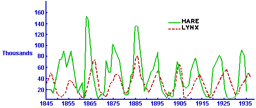
The lynx and hare population data depicted above are widely used because they come from essentially the longest-term population study in existence. The graph comes from Odum's Fundamentals of Ecology, which cites MacLulich's Fluctuations in the numbers of varying hare. The data itself comes from Hudson's Bay Company's records of pelts turned in for trading. Data could be skewed by disease outbreaks among the Native Americans doing much of the trapping during these years. Some authors caution that the data is actually a composition of several time series, with some lynx data missing, and should not be analyzed as a whole.

Models are inaccurate

Any model is an approximation of the complexities of reality. For example, the Lotka-Volterra model we are using ignores factors such as prey deaths from old age (if they don't get eaten), overgrazing (if there are too many), weather (essentially random), and other predators.

A brand-new model has yet unknown inaccuracies, and improving the model is likely to be one of the goals.

Implementations are inaccurate

At a minimum, an implementation is almost guaranteed to introduce some numerical inaccuracy. In the previous in-class example, we rounded populations at each step to integers. Using floating-point numbers only reduces the inaccuracy, as they still round numbers like 2 ⅓ to something like 2.3333333333333.

Larger inaccuracies resulting from algorithmic choices are also possible, and there is a whole field of measuring and reducing these. (See CAAM 353, Computational Numeric Analysis.)

Of course, an implementation could simply be wrong. Making mistakes, such as typing a formula incorrectly, is very easy to do, and hard to catch.

Understanding and Overcoming our Code's Inaccuracy

As you worked on the assignment due today, you almost certainly saw some anomalous behavior of our current algorithm. Populations should not ever go below zero. Populations should not fluctuate smoothly and then suddenly spike to infinity.

While it might not be obvious from the original problem wording, the Lotka-Volterra model's population changes are meant to be smooth curves. Instead, we interpreted them as annual changes, which seemed very natural from a biological perspective, but leads to a straight-line population change each year. This means our code does not accurately reflect the Lotka-Volterra model.

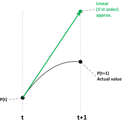
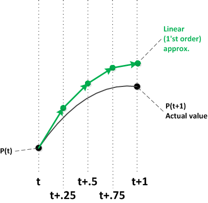
As illustrated by the above diagrams, one way to make this kind of approximation more accurate is to use smaller time intervals. Each line segment uses the curve's current slope. As the intervals get smaller and smaller, the resulting segments more closely approximate the curve.

Exercises — Improving the Code's Accuracy

What should our modified algorithm and code do? Overall, our purpose hasn't changed much. We still want to compute a series of populations, given the various inputs. Assuming a 5-year prediction, we previously generated someting like hare_pop = [(0, h0), (1, h1), (2, h2), (3, h3), (4, h4), (5, h5)] for some population values. Now we want multiple time steps per year. If we have just four time steps per year, we want to generate hare_pop = [(0, h0), (.25, h1), (.5, h2), (.75, h3), (1, h4), …, (4.75, h19), (5, h20)].

The specific code changes you need to make are as follows:

1. Copy your predator-prey code, creating a new version that you'll edit.
2. Add another parameter steps_per_year that represents how many time steps per year to make.
3. Update the documentation string to reflect the changes in the function behavior.
4. Edit the for statement. Instead of years getting the values 1, 2, …, years+1, we want to it to get values as illustrated above. Hint: Use the step argument for range().
5. Edit the formulas in the loop body. Each change in population needs to be divided by the number of time steps per year.

Test and debug.

Exercises — Experimenting with the Improved Code

As we increase the number of steps per year, the resulting population curves should converge upon the desired continuous model results. Experimentally, we would like to verify this, as well as determine how many time steps per year is good enough.

1. Choose a set of input rates that you'll keep constant in the following steps. It's best if you choose rates that are moderate — populations aren't neither too constant nor too rapidly changing.
2. Run your code with a variety of steps values, from one and higher. Compare the resulting plots.
   • As the number of steps per year get higher, do you see fewer anomalous data such as negative populations?
   • As the number of steps per year get higher, do the resulting curves converge? I.e., do they successively look like smoother versions of the same curve?
   • Above what number of steps do the resulting curves not change perceptibly?
3. Repeat with another set of rates. Do your answers change?

OK, here's a version of the updated predator-prey code, if you had trouble with the exercises above.

import simpleplot

def delta_h(h, l, hare_birth, hare_predation):
    """Returns the predicted annual change in hare population."""
    return h * hare_birth - h * l * hare_predation

def delta_l(h, l, lynx_birth, lynx_death):
    """Returns the predicted annual change in lynx population."""
    return h * l * lynx_birth - l * lynx_death

def populations(h, l, hare_birth, hare_predation, lynx_birth, lynx_death, years, steps_per_year):
    """Returns the predicted populations of hare and lynx for the given inputs."""
    hare_pop = [(0, h)]
    lynx_pop = [(0, l)]
    interval = 1 / steps_per_year

    for y in range(interval, years + 1, interval):
        h, l = (h + interval * delta_h(h, l, hare_birth, hare_predation),
                l + interval * delta_l(h, l, lynx_birth, lynx_death))

        hare_pop.append((y, h))
        lynx_pop.append((y, l))

    simpleplot.plot_lines("Hares and Lynx Populations", 600, 400,
                          "Years", "Population", [hare_pop, lynx_pop],
                          False, ["Hares", "Lynx"])

populations(100, 50, .4, .003, .004, .2, 50, 10)