Summary: An in-depth analysis of a simple coupled,two-level system that shows how the strength of the coupling perturbation affects the resulting repulsion of the eiqenvalues and the mixing of the original eigenstates.
A simple, two-level system is probably the simplest system that can be analyzed to see the effects of coupling between eigenstates. It is surprisingly rich problem with very interesting results that have connections to both classical and quantum physics applications.
Consider a system described by a 2x2 Hermitian matrix operator, M0. Such a system had two real eigenvalues, and when represented in the basis given by its eigenvectors, M0 is diagonal:
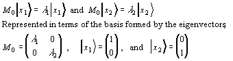
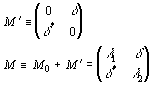
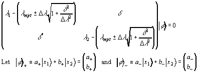
Now consider the addition of a perturbing operator, M', that consists purely of terms that couple the original eigenstates. That is, the perturbing operator does not add any constant offsets to the original eigenvalues because it has only off-diagonal elements. A new, perturbed operator, M, is the sum of M0, and M'.
The question is, in terms of the original eigenvalues and eigenvectors, what are the new eigenvalues and eigenvectors for the new perturbed operator, M?
The secular is equation is used to determine the eigenvalues:
Results
This analysis clearly shows a number of key features:
- The coupling between two unperturbed states will cause the new eigenvalues to be symmetrically split above and below the midpoint between the unperturbed values.
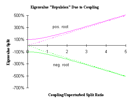
- It also shows that for Hermitian operators, the eigenvalues will be "repulsed" from each other, that is, the new values will be farther apart than the unperturbed values.
- For non-degenerate unperturbed systems, the "strength" of the splitting depends on the relative size of the coupling energy and the difference separation the unperturbed levels. The separation between the original eigenvalues determines a "characteristic size" to which everything is compared.
- For degenerate unperturbed systems, the effect of the perturbation is to break the degeneracy.
- A plot of the split in the eigenvalues induced by the coupling between the unperturbed states shows that the splitting of non-degenerate states asymptotically approaches the degenerate case. This is consistent with the idea that for large coupling to unperturbed split ratios, the unperturbed states are effectively degenerate.
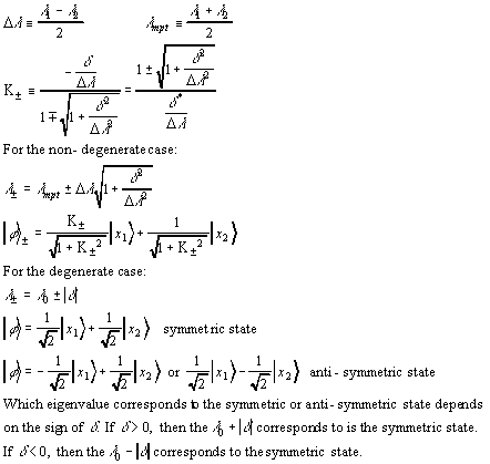
To solve for the eigenvectors, we simply plug the eigenvalues back into the eigenvalue equation. Below, we denote the coefficients associated with the positive and negative root solutions by "+" and "-" subscripts, respectively.
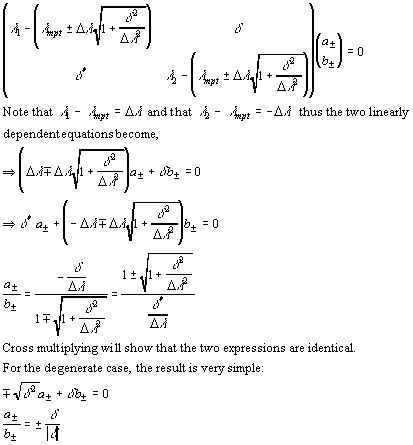
We can see several important properties of the wavevectors from the above analysis:
- In the degenerate case, we see the split into the symmetric (a± = b±) and anti-symmetric state (a± = -b±) states. Note that the symmetry of the state is not simply determined by the sign of the root used, but involves the sign of the coupling term as well.
- For the non-degenerate case, it is easier to see what is going on in the small perturbation limit:
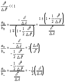
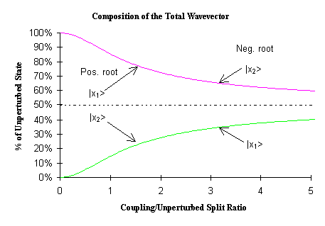
Here we see that the positive root solution is primarily composed of the |x1> state and the negative root solution is primarily composed of the |x2> state. - In a plot of the percentage composition of the total wave vector in terms of the two original states, we see that as the coupling to unperturbed splitting ratio gets large, the total composition asymptotically approaches the 50/50 makeup of the degenerate symmetric/anti-symmetric split:
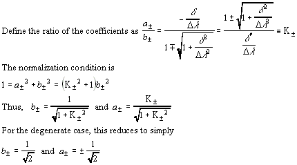
Note that for the degenerate case, the new eigenvectors are simply a 45° rotation from the original eigenvectors.
Conclusions
In summary, the new eigenvalues and eigenstates are given by
Notable features
- Any pure off-diagonal coupling will cause a symmetric repulsion of the eigenvalues.
- All effects can expressed in terms of the dimensionless ratio of the coupling term to the separation in the original eigenvalues, with the exception of the degenerate case, where the separation is zero.
- The large coupling limit approaches the degenerate case, both in terms of the eigenvalues and in terms of the composition of the new eigenvectors.
- The degenerate case and large coupling limit eigenstates are symmetric and antisymmetric states.
- In the perturbation limit where the coupling is very much smaller than the original eigenvalue separation, the non-degenerate eigenstates deviate only slightly from their original states. Likewise, the eigenvalues show a vanishingly small shift.
To do...
An in-depth analysis of the time-dependent eigenvectors will show that in the presence of a coupling field, a system initially prepared in a state corresponding to an original unperturbed eigenstate, will appear to oscillate back and forth between the two original eigenstates. This corresponds to the absorption and emission of a photon by a two-level atomic system. See the three spring problem module for the temporal analysis of a degenerate system.