Three Spring Problem

Summary: An in-depth analysis of the classic three spring problem from a perturbation theory perspective.

The classic 3-spring problem can provide a very rich insight into the nature of coupled resonant systems. By using a perturbation theory analysis and other insights from quantum mechanical systems on the problem, we can relate the results to other systems where resonant states (i.e. energy eigenstates/normal modes) in an unperturbed system are coupled together by some means. An example of this would be two energy states of an atom coupled by a electromagnetic field (photons).

Consider two identical masses, m, connected to opposite walls with identical springs with spring constants, k₀. The two masses are connected with a third spring with a spring constant, k₁.

In order to calculate the Lagrangian, we need to first calculate the kinetic and potential energies:

Lagrange's equations in generalized coordinates are:

= 0

This produces two coupled differential equations for x₁ and x₂, the "equations of motion", which could have been derived directly from F = ma:

Let us define the characteristic frequencies for the springs:

The differential equations thus become:

The normal modes each have a single harmonic time dependence for all the coordinates used to describe it and thus the x coordinates can be expressed as such (this amounts to the separation of position and time variables):

and thus, the differential equations can be rearranged into a matrix eigenvalue equation (after canceling the exponential time dependence out):

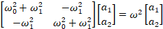
This is a degenerate coupled two level eigensystem problem. It is interesting to note that the system can be interpreted in two ways.

One is to consider the coupling spring as both coupling the unperturbed systems as well as adding an offset to them. That is, the matrix operator above consists of a diagonal unperturbed operator plus a perturbing operator that has both diagonal and off-diagonal terms:

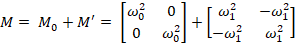
This view has the problem of making it difficult to identify the effect of the coupling on the unperturbed system because of the diagonal term offsets.

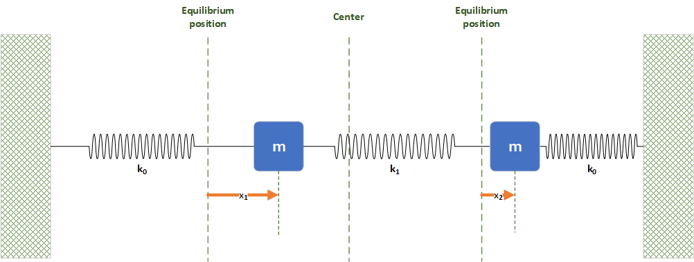
One the other hand, it may be easier to reconsider what really is the original, unperturbed system. Rather than consider the coupling spring to be an addition, consider a system where each mass initially has two restoring springs, one of spring constant k0 and the other with spring constant k1. This is equivalent to putting one finger down and immobilizing one of the masses. Thus we have two identical systems where we alternately immobilize the each mass. The unperturbed system thus has each mass with a net restoring spring of size k0+ k1. The perturbing operator thus has only off-diagonal terms:

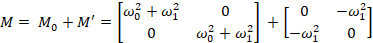
The analysis of this system is much cleaner and the splitting due to the coupling will be readily evident. See the module on solving such systems (Coupled Two Level Eigensystems).

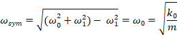
The two eigenstate ("normal mode") solutions can be characterized as a "symmetric" and "anti-symmetric" states whose eigenvalues and eigenstates are plus/minus splits from a central value where the amount of splitting is determined by the strength of the coupling spring (the off-diagonal terms in the above matrices). The stronger the coupling, the greater the splitting. Note that the split is NOT centered around the uncoupled but rather involves both sets of springs. Looking at the diagonal terms in the above matrix, we see that the central, unperturbed value is that which would occur if the center of the coupling spring was pinned and immovable. The diagonals of the non-coupled part of the matrix, ω² = ω₀² + ω₁² = (k₀+k₁)/m, tell us that each mass would move independently, governed by the simple sum of two springs.

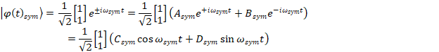
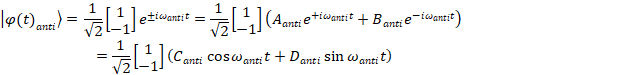
Note that both the positive and negative frequencies are solutions (technically, degenerate). This means that there are four unknown amplitude coefficients that need to be established by the boundary conditions. The four equations can be satisfied by specifying the initial values of the two coordinates as well as their initial time derivatives (velocities). This is normal for a second order differential equation.

Symmetric State

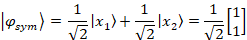
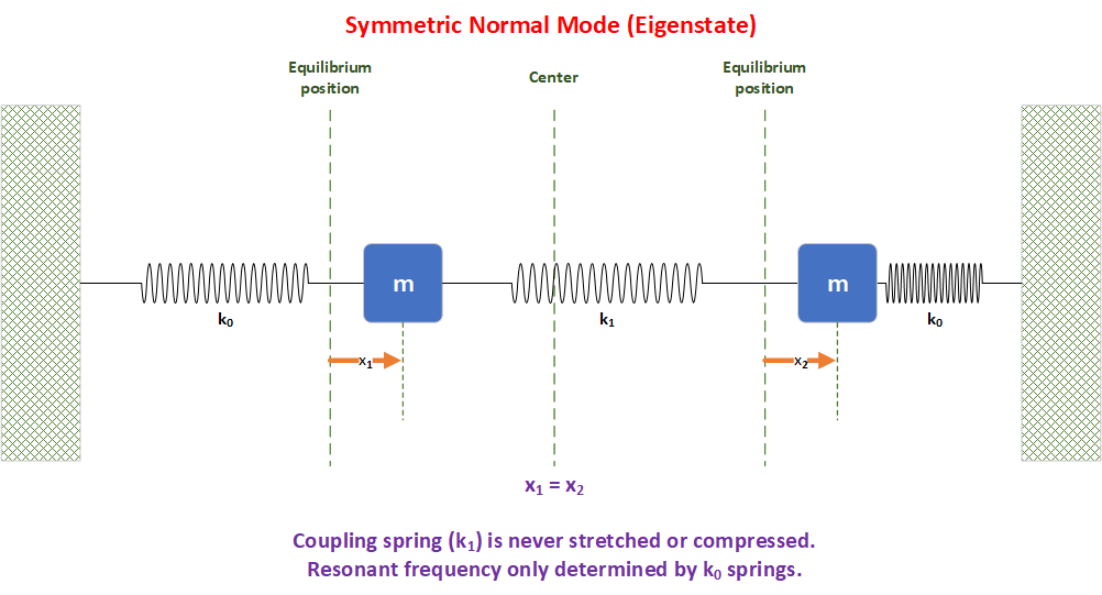
The symmetric eigenstate (symmetric "normal mode") has an eigenvalue (aka "resonant frequency") which is just that of the k₀ spring. The k₁ coupling spring does not contribute to the symmetric eigenvalue.

The x₁ and x₂ displacements of the masses are identical, meaning that they are moving together, always in the same direction:

The symmetric state can be interpreted as both masses moving exactly in phase to the left and right. The coupling spring does not get compressed or stretched at all in this case and has no effect on the masses. Hence the situation is as if each mass were affected only by one spring of spring constant, k₀.

Anti-Symmetric State

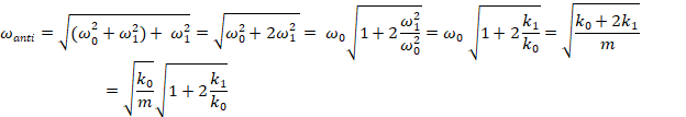
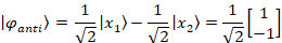
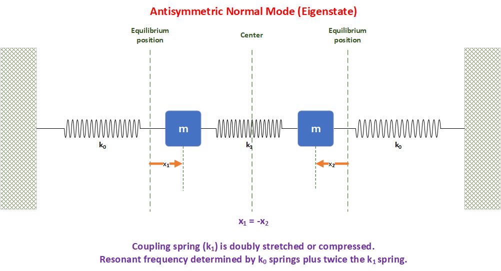
The anti-symmetric eigenstate (anti-symmetric "normal mode") has an eigenvalue (aka "resonant frequency") which is determined by the k₀ spring plus twice the k₁ coupling spring:

The x₁ and x₂ displacements of the masses are exact opposites of each other, meaning that they are always moving in exactly opposite directions:

The anti-symmetric state can be interpreted as both masses moving exactly in 180^o out-of-phase with each other. The coupling spring get doubly compressed or stretched at all in this case and thus has twice the effect on the masses as than if it were only connected to a single mass. Hence the situation is as if each mass were affected by one k₀ spring plus two k₁ springs.

The anti-symmetric state can be interpreted as each mass moving exactly 180° out of phase (hence the minus sign in the wavevector). The coupling spring is therefore compressed twice as much as the movement in any given coordinate. Thus it contributes an effectively larger restoring force, as if it had a spring constant that was twice as large. We can also see the advantage of the second viewpoint above on the unperturbed system. The new eigenvalues are a symmetric plus/minus split around (k₀+k₁)/m = ω₀²+ω₁², not k₀/m = ω₀².

Why Twice the Coupling Spring?

In the anti-symmetric eigenstate (normal mode), the center of the coupling spring, k₁, never moves. This begs the questions: "Isn't the anti-symmetric mode the equivalent of having nailed the middle of the coupling spring to the wall since it is not moving anyway? And in such, shouldn't the motion of the masses be as if they were independent from each other where each was connected to two springs, a k₀ and a k₁ spring? Wouldn't that make the resonant frequency just the square root of (k₀+k₁)/m, not the square root of (k₀+2·k₁)/m?

The resolution of this conundrum lies in a misconception of what happens to a spring when it is cut in half. It is tempting to believe that if spring with a spring constant, k, is cut in half, the result would be two springs of spring constant k. But that's not actually what happens.

A spring's behavior is defined by its characteristic of a restoring force that is linear in the displacement of the end of the spring from its equilibrium (resting) position: F = -k·d. When a spring is stretched (a uniformly coiled spring is assumed here) by a total displacement, d, that stretching is spread across the entire length of the spring. Thus only half of the displacement is being applied across each half of the spring for any given total displacement of the whole spring..

But if the spring is cut in half and we stretch that half-spring by the same total displacement, d, that is an equivalent amount of stretching for the whole spring of 2·d, i.e. twice that was applied to the whole spring! The restoring force of the half-spring for any total displacement, d, is actually twice that of the whole spring for the same displacement. This means that the half-spring's actual spring constant is twice that of the whole spring or 2·k!

Nailing the center of the coupling spring down and making it immovable is thus equivalent to replacing the one coupling spring with two independent springs of twice the original spring constant and the individual masses thus move as if they were connect to springs of k₀ and 2·k₁, which is the result we calculated above.

Non-eigenstate time evolution

How would the coupled system behave if it was originally prepared in one of the unperturbed eigenstates, which are NOT eigenstates of the coupled system?

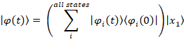
The composition of a time evolving state in terms of the new eigenstates can be expressed via its overlap (Completeness Theorem with time dependence). Half the initial conditions can be satisfied by setting the expansion coefficients at t=0 (the initial velocity still needs to be satisfied):

Suppose the initial state is a unit displacement in only one of the original coordinates, i.e. one mass pulled to one side and the other at its central equilibrium point.

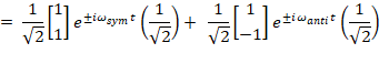
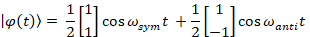
If we want the initial velocity to be zero, then the exponentials reduce to the cosine solutions only:

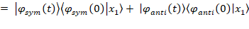
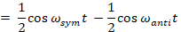
To see the time evolution of a particular coordinate, we need to look at the projection along its direction at time, t:

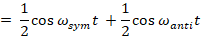
Using the trigonometric identity

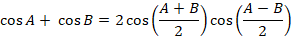
We get

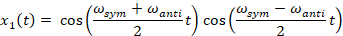
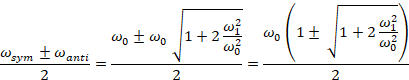
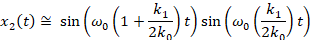
If k₁ << k₀, i.e. the coupling spring is very weak compared with the main springs, then the following approximation holds:

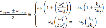
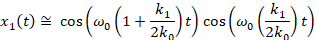
The motion of the x₁ mass is a vibration at approximately the original, unperturbed frequence but shifted slightly by an amount determined by the ratio of the coupling to original spring strengths. However the amplitude of that slightly perturbed oscillation is modulated at a much lower frequency which is a fraction of the unperturbed frequency determined by the ratio of the coupling to original spring strengths.

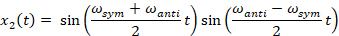
For the other coordinate, the process is the same:

Using the trigonometric identity

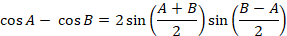
We get

If k₁ << k₀, i.e. the coupling spring is very weak compared with the main springs, then the following approximation holds:

We see that the motion of the x₂ mass is 90^o out-of-phase with the x₁ mass but at the same slightly shifted base frequency and amplitude modulation frequence. Note that the slow amplitude modulation is also 90^o out-of-phase with the x₁ mass's amplitude modulation.

Conclusion for lightly-coupled masses:

If the system is initialized with only an x₁ mass displacement and zero initial velocity, the x₁ mass will appear to oscillate at a frequency only slightly, perhaps even imperceptibly, off from the single spring (k₀) frequency. But the amplitude of that oscillation will periodically rise and fall. On the other hand, the x₂ mass will appear also appear to oscillate at the same near-k₀-determined frequency but completely out-of-phase with the x₁ mass. As the amplitude of the x₁oscillations dies, the amplitude of the x₂ oscillations grows and vice versa. Energy is being transferred back and forth between the two masses.

This energy transfer between the two masses is due to neither sole x₁ displacement nor sole x₂ being eigenstates of the coupled system. Since the eigenstate resonant frequencies (eigenvalues) are split apart by the coupling and thus not identical, the net result is a "beating" between the eigenstates that form the state in which the system was prepared (i.e. a sole displacement in the x₁ direction).

We can clearly see that the solutions consist of modulated cosine and sine waves. The fundamental frequency is approximately equal to the unperturbed frequency for small coupling. The modulation envelope frequency is equal to the coupling frequency. The change in the fundamental frequency, given by the ω₁/ω₀ factor, is a "frequency pulling" effect that shows up in the real world as changes to oscillator frequencies in the presence of parasitic couplings between components.

While energy appears to be flowing back and forth between the |x1> and |x2> states, it is really just a beating between the different frequencies of the two stationary eigenstates.

Relationship to atomic systems with photons

Note that this system is conceptually similar to two atomic levels coupled by a harmonic photon field. This will cause an electron in the lower energy state to be absorbed and jump to the higher energy state. After a while though, the photon field will cause a stimulated emission and the electron will drop to the lower state.

The other effect that we see here is that a perturbing field will split degenerate energy levels into symmetric and anti-symmetric states. This one of the basic mechanisms for the formation of energy bandgaps in semiconductors.

Something to think about...

Suppose all three springs had different spring constants. This would break the initial degeneracy of the uncoupled solutions. In this case, the 3 spring problem would reduce down exactly to a coupled two-level systems problem, which starts off with split energy levels and is split further by the coupling.