Comp360/560 Lab3 : Ray Tracing

First Milestone - April 02, 2019, 11:59pm
Final Submission - April 14, 2019, 6:00pm

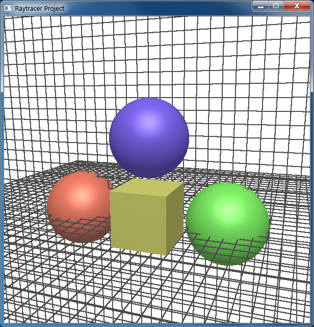
Figure 1: Modeling window

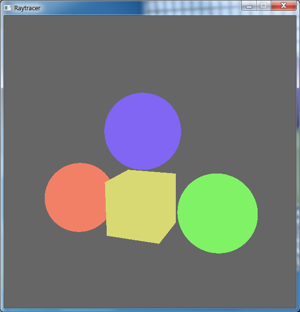
Figure 2: Ray-tracing window

1  Overview

2  Project Overview

• complete the sphere and box intersection code,
• fill out the rest of the code for ray-tracing other objects,
• write a few user-interface/application enhancements to the given framework.

2.1  First Milestone (40 points)

• Implement the ray-sphere intersection code using the algorithm in the textbook. (6 points)
• Compute face normals at ray-box intersections (computing intersection points already done for you). (4 points)
• Implement the ray-tracing illumination model. (6 points)
• Implement shadow effects, reflection, refraction, and transparency. (20 points)
• Implement the ability to dynamically add spheres and boxes to the scene as well as remove them from the scene. (4 points)
• Ray-trace scenes containing any number of light sources, spheres, and boxes. The other object types are not required at this time.

2.2  Final Submission (52 points)

• Render polygonal versions (using OpenGL) of ellipsoids, cylinders, and cones. (12 points)
• Ray-trace ellipsoids, cylinders, and cones. This requires you to compute ray-object intersections and normals at the intersections. (32 points)
• Implement the ability to dynamically add and remove any object from the scene. (4 points)
• Implement the ability to save the current scene into a file in the format as described in "Scene File Format". (4 points)
• Ray-trace scenes containing any number of light sources and objects (but not too many).

2.3  Scene Files/Pretty Pictures (28 points)

2.4  Extra Credit (20 points)

• Ray-trace a torus (see textbook). (12 points)
• Add GUI for interactive adding/removing/manipulating light sources. (8 points)

3  Program Controls

• See the course textbook for the algorithms and calculations used in recursive ray tracing. For alternative presentations, you might also want to look at Foley and van Dam's book or on the web. You may use alternatives to help you understand ray tracing, but only the algorithm presented in the course textbook will be accepted. For example, to ray trace the ellipsoid, one approach is to solve the implicit equations of the ellipsoid and the ray. However, this approach is not what we are looking for.
• If we consider the presentation in the textbook, intersecting a ray with a basic geometric shape can be reduced to intersecting with some canonical shape. For example, intersecting a ray with an ellipsoid can be reduced to intersecting a ray with a unit sphere (centered at the origin). An ellipsoid can be viewed as the image of an affine transformation applied to the unit sphere. Therefore, if we apply the inverse transformation to the ray, compute the intersection between the transformed ray and the unit sphere, and forward-transform the intersection point, then we will have the intersection point on the ellipsoid. This approach should be the basis for all of your intersection code (please look at the box example in the given code). Here is a mathematica file that illustrates this intersection algorithm. Normals are handled similarly.
• Remember, when a ray intersects a reflective or refractive surface, rays are traced recursively from the intersection point.
• Shadow rays are NOT refracted. The contribution factor of a light source (along a particular shadow ray) is a real number within [0,1]. If a shadow ray hits an object with a positive transparency coefficient t, scale the factor by t and continue tracing the shadow ray.
• Your program may assume that input files are well-formed. Still, be careful when you modify the files directly.
• You should treat the transparency as a weight that you apply to your refracted ray in the same way you use the reflective coefficients to weigh the reflected ray.
• The general outline for the trace() function can be found here:

  TraceResult trace(Ray r):
     hit = check if any intersection point has be found
     if hit:
        // first add the ambient contribution, independent of the light sources
        result = ambient_color * ambient_light
        for each light source L:
            shadow = compute the shadow factor (wrt L) as described on this project page
            diffuse = compute the diffuse component wrt L
            specular = compute the specular component wrt L
            result += shadow * (diffuse*diffuse_coeff*light_color + specular*specular_coeff*light_color)
  
        if reflection_coeff > 0:
            reflect = compute color of the reflected ray as described in the book (call trace again)
        if transparency > 0:
            refract = compute color of the refracted ray as described in the book (call trace again)
  
        result += reflection_coeff*reflect + transparency*refract
  
        // you should cap each channel of your result to 1.
  
        return result
     return no hit
  

• You may assume that the refraction index of air is 1.
• Let L be the vector from the intersection point to the light source, and let N be the normal at the intersection point. You only want to add the specular and diffuse components if (L·N) > 0.
• The gray background color in the given code is only for demonstration. You should replace the grey background with a black background.
• To compute the normals for a deformed shape, you would need to multiply the undeformed normal by the inverse transpose of the deformation matrix. Please refer to the textbook for more details.
• A normal is a 3D vector so its fourth component is 0. One common mistake is that when the deformed normal is found, the fourth component is not 0, and when you try to normalize that vector, its magnitude is incorrect. Make sure when you are normalizing a vector in 3D, that the fourth component of the homogenization of the vector is 0.
• To debug or visualize normal vectors, you may use their coordinates as actual object colors. In this case, you may have to adjust value ranges from [-1,1] to [0,1]. Then the colors should vary smoothly on smooth surfaces and correspond to correct directions. For example, points on the surface facing the positive x-direction might appear red if we map the x-coordinate of the normal to red in RGB.
• Since rendering a complex scene can take several minutes, you are advised to ray-trace complex scenes in "Release Mode" rather than "Debug Mode." Also run the project by pressing Ctrl + F5 rather than F5. To demonstrate the difference, the TA's ray tracer takes 146s (2.5min) in "Release Mode" and 557s (9min) in "Debug Mode" to render one particular complex scene.
• Following the last point, try to focus on code speed besides code readability.
• Try not to interact with the running program while it is ray-tracing your scene.
• When you write code for ray-object intersection, use inverse deformation matrices that are already computed rather than inverting the matrices directly (see the box example).
• Look for "TODO" in code comments for where you will have to add more code. See also "NOTE."
• To remind the user, including the TA, print to the console messages about how to add or remove objects.
• Common and potential mistakes:
  • forget to reset homogeneous coordinates correctly (1 for points, 0 for vectors, as mentioned above),
  • normalize some vectors when you shouldn't (e.g., ray directions),
  • forget to normalize vectors when you should (e.g., face normals),
  • forget to update inverse transformation matrices (e.g., _imat),
  • forget to update inner matrices with updateTransform(), or update at a wrong time,
  • mark ray-tracing results as hit/miss incorrectly,
  • recursively ray-trace at the same point (of the same object),
  • use exact equality for floating-point numbers (precision errors).

4.3.2  Operator

• An operator is the axis that appears at the center of a geometric object when you select the object. Its function is to allow direct translation and rotation in the modeling window. When you press shift while an object is selected, the axis will turn into three circles, which denote the ability to perform direct rotation.
  
  Each operator has two operands: primary and secondary. Every time an operator is moved or rotated, the operands are notified that an action has been performed on the operator (see Operator.h). In the given code, the primary operand is just a geometric object (or Geometry, like a Sphere). The secondary operand is the property window. This means that every time an operator is translated or rotated, the associated Geometry and fields in the property window are also changed. These changes correspond to the rotate() and translate() functions in ShadeAndShapes.cpp and PropertyWindow.cpp. You have to fill out these functions for each of the remaining geometric object in ShadeAndShapes.cpp (the box and the sphere have been done for you).
• Now we can consider adding or removing geometric objects from the scene. If you look at the function prepScene(), you can observe that one operator is created for each geometric object. Furthermore, there is a link from geometry to operator (the _geom2op map). If we are adding or removing objects, we need to update the mapping from geometry to operator. This update can be done just by calling prepScene() again, or you can write a more efficient version.
• Finally, the following is something to watch out for when you are writing your code. Note that an operator only comes into play when a geometric object is selected. When an object is selected, we need to activate the operator in the current editing state. When an object is de-selected, we need to deactivate the operator in the current editing state.
  
  When you are deleting an object that is selected (and in the editing mode), you will need to deactivate that operator. This deactivation code should be similar to, if not the same as, the code in the INPUT_SELECTING section of the mouseEvent() function in MainWindow.cpp.

4.3.3  Code Base

• ArcBall.h/cpp
  • Camera manipulator.
  • No need to change anything.
• Common.h
  • Some code for common definitions. Utility functions.
• Geometry.h/cpp
  • Defines the base class for the different shapes.
  • Visitor for the different geometric shapes.
  • Some geometry-utility functions defined in GeometryUtils.
• MainWindow.h/cpp
  • Main window. Modeling window.
  • Hooks operators to geometries.
  • Contains logic for program controls like viewing, operators, and ray tracing.
  • Need to add dynamic add/delete feature.
  • Remember to connect operators to geometries when dynamically creating new geometries. Similarly, disconnect when deleting.
  • Probably need to heavily modify this to add other UI features.
• Matrix.h
  • Contains Vector and Matrix definitions. Use Vec3, Pt3, and Mat4 in your program. The affine representation for each is just an extension of the description in the Iterated Function Systems (Section 3.1.2)
• Operator.h
  • Operator is the object that allows direct position/rotation manipulation in the modeling window. It shows up as three axes or three rings. You can use the operator to translate or rotate your geometry directly in the modeling window.
  • Shouldn't need to add anything here.
• PropertyWindow.h/cpp
  • Code for the property window that pops up when an object is selected.
  • GeometryUpdater will update each geometry given new input from the Property window.
  • WidgetUpdater will update the Property window given new values from the geometry.
  • Need to fill out the GeometryUpdater and the WidgetUpdater for other shapes.
• Raytracer.h/cpp
  • Contains actual ray tracing code.
  • Need to write recursive ray tracing in the trace() function.
  • Need to implement illumination.
• RaytracerViewer.h/cpp
  • The viewing window for the ray tracing result.
  • Shouldn't need to add anything here.
• Renderer.h
  • Base class for zbuffer and ray tracing output.
• Scene.h/cpp
  • Contains definition for a scene, which contains geometries, lights, and materials.
  • ReadSceneObjectVisitor helps reading object description from a file.
  • readScene() reads a scene from a file.
  • Fill out removeObject() in Scene.h.
  • Fill out WriteSceneObjectVisitor and ReadSceneObjectVisitor for other shapes.
• ShadeAndShapes.h/cpp
  • Contains definition for light and materials.
  • Definitions for all the shapes
  • Contains Intersector, which is a visitor for the shapes that performs intersection.
  • Need to fill out the member fields (axes, lengths) for each of the shapes.
  • Need to define how Operator functions affect each shape (look at Sphere and Box for reference).
  • Need to fill out the intersection code (visit()) for each of the shapes.
• ZBufferRenderer.h/cpp
  • Contains rendering code for polygonal rendering.
  • Need to fill out the ZBufferVisitor for the other shapes.

5  What To Turn In

• The names of you and your partner (or only your name if working alone),
• A brief overview of any major modification to the code,
• Information about your scene files,
• Any known bugs or incomplete features,
• Any other implementation details you think your grader should know.

6  Scene File Format

// Lighting
0.3 0.3 0.3    // R, G, B of ambient color
1              // Number of light sources
0 5 5          // x, y, z position of the first light source
1 1 1          // Color of the first light source
// More lights

// Objects
2     // Number of objects

// First object
sphere         // Type
0 0 0          // x, y, z coordinates of center of the sphere
1.5            // radius of the sphere
0.1 0.1 0.1    // Ambient coefficient
0.45 0.45 0.45 // Diffuse coefficient
0.5 0.5 0.5    // Specular coefficient
5              // Specular exponent
0.5            // Reflection coefficient
0.1            // Transparency coefficient
1.6            // Index of refraction

// Second object
box            // Type
0 0 0          // x, y, z coordinates of corner of box
1 0 0          // Normalized vector of the direction of Length (vl)
0 1 0          // Normalized vector of the direction of Width (vw).
0 0 1          // Normalized vector of the direction of Height (vh).
.5 .5 1        // The Length, Width, and Height of the box, in floats.
0.1 0.1 0.1    // Ambient coefficient
0.45 0.45 0.45 // Diffuse coefficient
0.5 0.5 0.5    // Specular coefficient
5              // Specular exponent
0.5            // Reflection coefficient
0.1            // Transparency coefficient
1.1            // Index of refraction

1 0 0 0 0 1 0 0 0 0 1 0 0 0 0 1 0 0 2  // The camera description