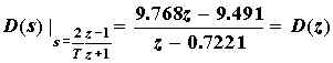
Discrete-time Controller Design

The dynamics of the system can now be incorporated into the design of a discrete-time compensator, D(z), that will allow control of the output variable, namely, the position of the load shaft, Q(s). The control diagram of Figure 1 below applies. Digital to analog conversion is modeled as a zero order hold (zoh), the transfer function G_h(s) of which is shown in the diagram. The error signal R(s)-Q(s) is sampled at rate T. The design of the controller is carried out in the s*-domain using the bilinear transform (the superscript * indicates that this domain corresponds to the bilinear transform). The following steps summarize the process:

1. select sampling period T
2. discretize zoh and plant, G_hG_p(z)
3. compute inverse bilinear transform of zoh and plant, G_hG_p(s*)
4. design controller in the s-domain, D(s*)
5. compute bilinear tranform of controller, D(z)
6. implement design

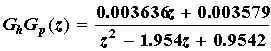
Following a common rule, sampling rate T is set to 0.1*t_r, where t_r is the rise time of the step response (Figure 2, modeling section), and t_r=0.1 s; then T=0.01 s. Due to sampling the cascade combination of the zoh and the plant is discretized. The resulting transfer function is

.

The design of the controller will be based on the inverse bilinear tranform of G_hG_p(z). Bilinear tranformation is required because design techniques in the analog domain are available. Thus,

.

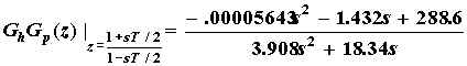The frequency response of G_hG_p(s*) is ploted in Figure 2 (Bode plot). The controller will aim to increase the phase margin. The effect will be an increase in the relative stability of the system.

Phase Lead Controller Design

Phase-lead compensation introduces a phase lead, which is a stabilizing effect. It also increases system bandwidth, resulting in a faster time response. On the negative side the compensator introduces noise because it increases high-frequency gain. The general form of the controller transfer function is

where a and b are computed according to

.

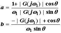w₁ is the frequency at which the compensated system has a phase margin of f_m, and q=180+f_m+ <G(jw₁). G(jw) is the frequency response of G_hG_p(s*) (Figure 2). The compensated response is shown in Figure 3 (red lines). Clearly, both the magnitude and phase have shifted to the right, generating the desired effect of increased stability margins. The designed controller is

.

Taking the bilinear transform, we get

.

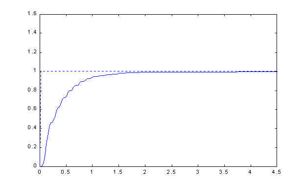
(for a listing of the Matlab code used in the design, click here). The frequency response of the digital controller is shown in Figure 4. Clearly the controller has the characteristics of a high pass filter. The step response of the compensated system is shown in Figure 5. Comparison with Figure 2 of the modeling section reveals that the controller is successful in improving the relative stability of the system. The ripples visible in the transient part of the response are due to amplified noise.

Figure 1: Block diagram of compensated system with discrete-time controller D(z)

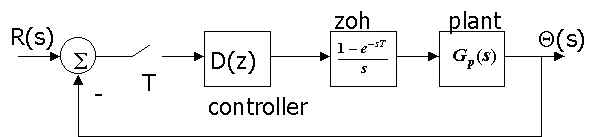
Figure 2: Frequency response of G_hG_p(jw)

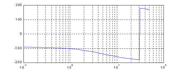
Figure 3: Frequency response of G_hG_p(jw)D(jw) (in red, uncompensated response in blue)

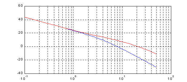
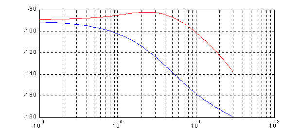
Figure 4: Frequency response of D(e^jw)

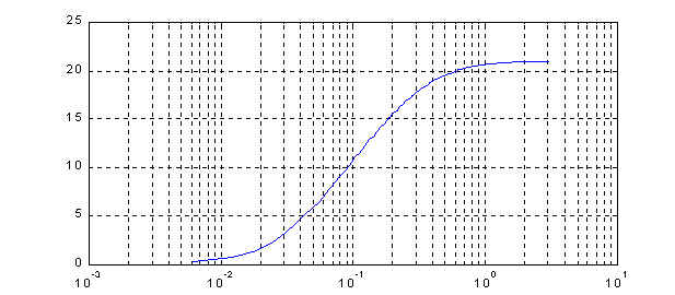
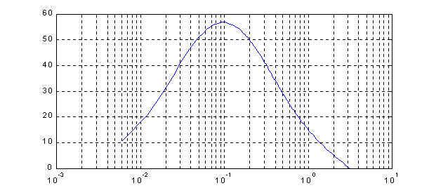
Figure 5: Step response of compensated system