System Modeling and Identification

The motion of the system can be described completely by a single degree of freedom, quantified by the angular displacement of the load shaft, q(t)(the belts connecting the inertia disks are assumed to be rigid, see system description). If Q(s) is the Laplace transform of the load angle and R(s) the desired position (input), then the closed loop transfer function of the system (see Figure 1 below) can be modeled as a prototype 2^nd order system,

where w_n is the natural frequency and z the damping ratio. The transfer function of the plant Gp(s) is given by

.

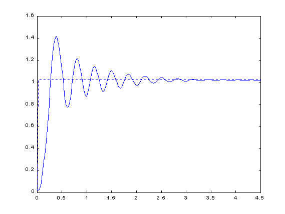
The numerical values of both the natural frequency w_n and damping ratio z can be determined by examining the system response to a step input. Input R(s)=1/s is the reference trajectory, a unit step in this case. The step response is measured and plotted in Figure 2. The maximum overshoot is 1.41 rad, occuring at time 0.38 s. Model parameters can be determined from the following formulas,

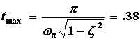
The natural frequency is w_n=8.59 rad/s and the damping ratio z=0.273. The plant transfer function is

.

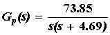The purpose of the next section is to design a controller that will improve on the relative stability of the system. Although the uncontrolled system is stable, its step response exhibits large overshoot and subsequent oscillations do not subside until after 3 s (Figure 2 ). It should be pointed out here that the second order model has a step response that decays faster than the actual response shown in the figure. A third order model would have been a better aproximation of the system behavior.

Figure 1: Block diagram of uncompensated system

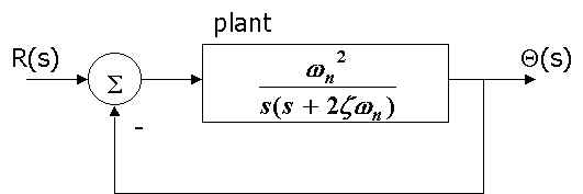
Figure 2: Unit step response of uncompensated system