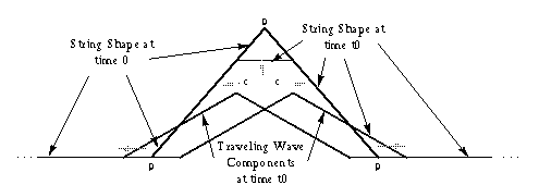
 image taken from
p.3,
Reference [1]
 image taken from
p.3,
Reference [1]
where we can see that the traveling wave is composed of two components (a left-going wave and a right-going wave). From Physics, we know that the solution to this one-dimensinal traveling wave is
where yr and yl denote the right and left going waves, respectively.
(note: the brackets [ ] shows that the signals are DISCRETE.)
This can be implemented by the following model:
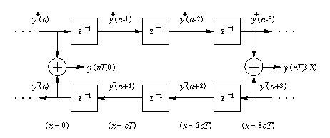
Digital Implementation of an IDEAL, LOSSLESS traveling wave
On this diagram, the top rail represents the right-going traveling wave in (eqn 2). Each of the z^(-1) corresponds to the delay in (eqn 2). The bottom rail, on the other hand, represents the left-going traveling wave. We can get an output at any discrete instant (spatially and temporally) by summing up the top and bottom rail outputs at that point.
In the real world, however, there are losses as the wave travels on the string. Therefore, to make the above digital simulation more realistic, we modify it to the following model:
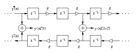
Digital Implementation of an IDEAL, LOSSY traveling wave
This model is similar to the first model, with one slight modification--we put losses g next to each delay element. Physically, this means that as the wave travels along the string, it experiences losses along the string.

Digital Implementation of a string with consolidated losses and
delays
In this model, we put all the delays together on the top rail and all the losses on the bottom rail. The advantage of doing this is that we will get a better result because we are not rounding off the numbers 100 times like before. Also, this is a lot simpler to implement.
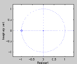 z-plane design of lowpass filter
If we want to make the frequency response = 1 at w=0, we need:
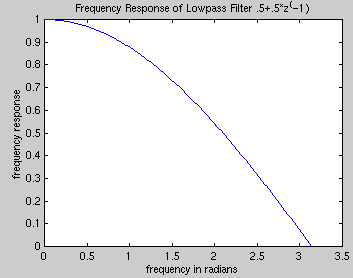 .5 + .5*z^(-1)
After generating the note A (440Hz) using pluck.cc and passing the .snd file through MABLAB to generate the graphs and sound, we obtained the following results:
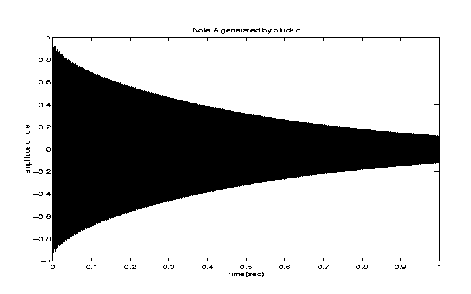 Note A (1 second)
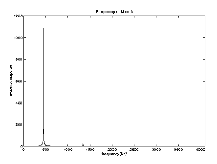 Frequency Response of Note
A
Note that the frequency response peaks at around 440Hz (note A).
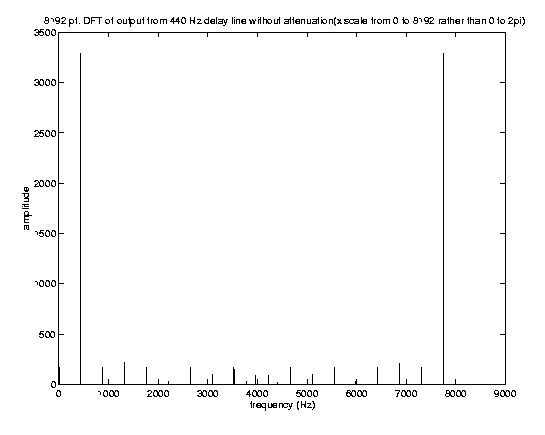
For experimentation, we tried to design different loss filters. We moved the location of the ZERO of a + b*z^(-1) to different places to implement different lowpass filters. We tried to place the zero at z=-0.1 to decrease attenuation. As expected, note A took a lot longer to die out when z=-0.1. We even rewrite pluck.cc to eliminate ATTENUATION (the lowpass filter). When we did that, the note never died out, as expected. From the frequency spectrum plot below, we can see that when we do not have attenuation, note A is consisted of only certain discrete frequencies. This is in big contrast to the frequency spectrum WITH attenuation, where we see that note A is consisted of all sorts of frequencies.
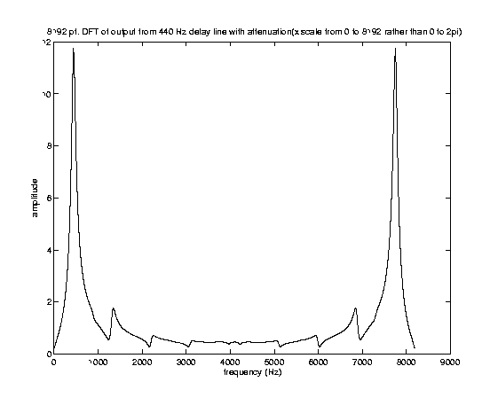
DFT of output from 440Hz Delay Line without Attenuation.
DFT of output from 440Hz Delay Line with Attenuation.
We have discovered something interesting through trying out different sampling rates and zero locations. For a fix desired musical note frequency (for example, note A at 440Hz), we know that w = OMEGA/fs, where OMEGA stands for the analog frequency, w stands for the discrete frequency, and fs stands for the sampling frequency. If we fixed our lowpass loss filter design to .5+.5*z^(-1), by changing the samling rate fs, we got different levels of attenuation. This is because different sampling rates give us different w's. As sampling frequency INCREASES, w DECREASES for a given OMEGA. A lower w corresponds to a lower frequency response magnitude for a fixed lowpass filter design. This lower frequency response magnitude causes the same note (say, 440Hz), to die off a lot faster.
We composed some songs by combining notes together. Mary Had a Little Lamb was a very successful song that we wrote using pluck.cc. This is because the three notes that we used for this song were B(494.7Hz), A(440Hz), and G(392.4Hz), which were at relatively LOW frequencies, and hence tuning was not bad. We also wrote Twinkle Twinkle Little Star but that was not very successful, because we wrote it in G major, which contains the note D at 602.7Hz. This note sounded identical to E (665.3Hz) because of problems that we mentioned in the Fractional Delay section.
In addition, we were able to combine notes together and play different intervals/chords. Once again, however, notes at high frequencies are not always in tune.