|
|
| 2D Filtering Concepts |
Brought to you by Team Phantom
Cruiser and the Power of Steam
|
|
|
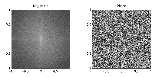
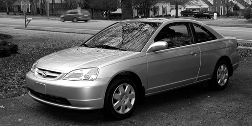
| | Top: Original image. Bottom: Spectrum of original image. |
Above we have both an image and it's spectral representation. But
before we can work with filtering this image, we must first examine
what this frequency content indicates. In a time-based signal, a low frequency signal is one
which changes slowly, whereas a high frequency signal has a more rapid
change. To extend this concept to a spatial signal, it is easy to see
that low-frequency data occurs where intensity values change slowly,
i.e. a smooth gradient, and high frequencies equate to a rapid change
in intensity, i.e. a sharp edge. Armed with these concepts, we can
now anticipate the results of filtering an image.
|
|

| | Top: Original image. Bottom: Image filtered with
ideal lowpass filter on Y axis, normalized cutoff frequency .15. X
axis is an allpass. |
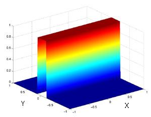
When we try to use an rectangular lowpass filter in
the Y direction two things are illustrated. First, an ideal
rectangular filter cannot be used because it creates "ringing"
artifacts, the same as in a one-dimensional transform. The second
and more important realization is that a filter varying
only in the Y frequency direction, and equal across all X, has its effects only
in the Y direction of the image. We expect this from the rotation property, and from this we can
infer, properly it turns out, that a filter is just as seperable as the
transform, and therefore the direction of a filter will be the
direction of its effect. Notice
the way the shadows ripple up and down from horizonal lines in the
original image, whereas vertical lines such as the edge of the car
door are unaffected.
|