|
LPC has been widely used in speech recognition systems. In this section we describe the method we implemented for recognition of numbers 1 to 5, using LPC cepstral coefficients. We followed the basic ideas proposed by Markel et al. [2], Papamichalis [5] and Rabiner [6]. Figure 1 shows a block diagram of the speech recognition system. The basic steps in the processing of each word are the following: Figure 1:  |
| 1. Pre-emphasis The speech signal (here, also refereed as {\it word}), s(n), is filtered with a first-order FIR filter to spectrally flatten the signal. We used one of the most widely used preemphasis filter of the form  where a=15/16. Appendix A shows an example of a word `three' preemphasized. The signal was sampled at a frequency of 8 kHz. Observe that the filter removes the DC component of the signal. |
| 2. Normalization After preemphasis, each word has it's energy normalized. Based on the energy distribution along the temporal axis, it is computed the center of gravity, and this information is used as reference for temporal alignment of the words. Appendix B shows examples of temporal alignment. The energy of each word was computed using 60 non overlapping windows. The program is in Appendix C. |
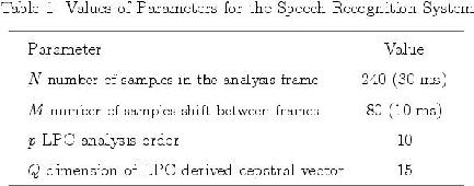
| 3. Frame Blocking The preemphasized speech signal, s^[n], is blocked into frames of N samples, with adjacent frames being separated by M samples. Table 1 gives the values used for N and M. If we denote the l:th frame of speech by xl[n], and there are L frames, then  where n=0,1,...,N-1, and l=0,1,...,L-1.  |
| 4. Windowing Each individual frame is windowed to minimize the signal discontinuities at the borders of each frame. If the window is defined as w[n], 0 < n < N-1, then the windowed signal is  where 0 < n < N-1. We used a Hamming window, a typical window used for the autocorrelation method of LPC. Appendix D shows an example of a windowed frame. Observe the borders of the signal. |
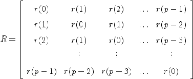
| 5. LPC Parameters The next processing step is the LPC analysis using the autocorrelation method of order p. In matrix form,  where  is the autocorrelation vector,  is the filter coefficients vector, and  is the Toeplitz autocorrelation matrix. This matrix is nonsigular and gives the solution,  The autocorrelation method is very effective in speech processing [5], [6]. |
| 6. LPC Parameter Conversion to Cepstral Coefficients The LPC cepstral coefficients, c_m, are a very important LPC parameter used in speech recognition. They can be derived directly from the set of LPC coefficients a_i for i=1,...,p, using the recursion  where 1 < m < p, and  where m > p. The last equation is not correct in reference [6] and was derived using [5]. The cepstral coefficients, which are the coefficients of the Fourier transform representation of the log magnitude of the spectrum, have beem shown to be more robust for speech recognition than the LPC coefficients. Generally, it is used a cepstral representation with Q > p coefficients, where Q~(3/2)p. |
| 7. Cepstral Distance The cepstral coefficients provide an efficient computation of the log-spectral distance of two frames [5]. For LPC models that represent smoothed envelopes of the speech spectra, it is usually used a truncated number of cepstral coefficients. In our work we used a truncated cepstral distance [6] defined by  |
| 8. Training and Classification In the last part, we build a codebook of cepstral coefficients. Each one of the five classes of words (numbers one to five) is represented by 58 vectors, each one with 15 coefficients. Each vector represents a frame of a class. One routine in Matlab is used to compute the average vector for each frame based on sets of 30 words for each class. The codebook is stored and used in the classification routine. The program used in the training stage is in Appendix E. The classification procedure for arbitrary spectral vectors is basically a full search through the codebook to find the `best' match. A classification routine in Matlab, computes the cepstral coefficients of the unknown input word. After that, it computes the distance between each vector of the input word and the corresponding vector in the codebook. The input vector is classified with the number associated with the class that gives the minimum total distance. The classification program is in Appendix F. The program in Appendix G was used to play the matlab data files. |
