| Formant Trajectory method |
Introduction Power method Formant Trajectory Cepstrum method Result Conclusions Future work Bibliography |
|
In this method, you divide the signal into time blocks. You then take these blocks and determine an AR model for each block, and choose the first 3 positive frequencies for the poles as the formant frequencies. You obtain this information for all of the time windows. Then you compare this information to the models for the different words to determine what word you are looking at.
|
|
Before the signal can be broken into parts it is pre-emphasized with a high pass filter. This filter emphasizes the upper formant frequencies. After this is done, the signals were aligned in time by searching for the first main spike and then using that point as the start of the signal. What this did was to assure that there were not any gaps between the beginning of the signal and the beginning of the word. Since the time signal varies over time, you need to break the signal into small intervals of time, about 30 ms. Over this time period you will assume that the signal remains stationary. In the model that we created, we used 30 ms windows, and then we windowed with a hamming window. The windows were then shifted by 10 ms. Each word had a total of 42 windows. This window size was chosen because that same size was used in several different references.(2)(3) |
|
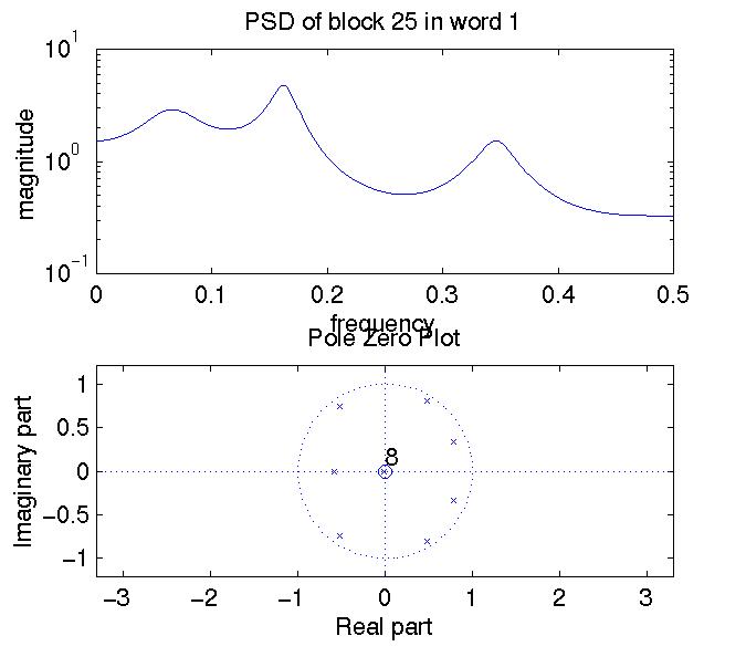
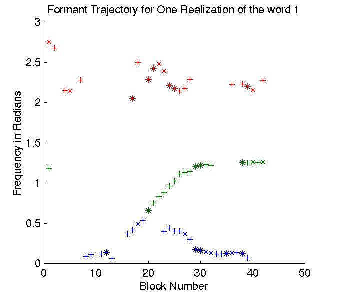
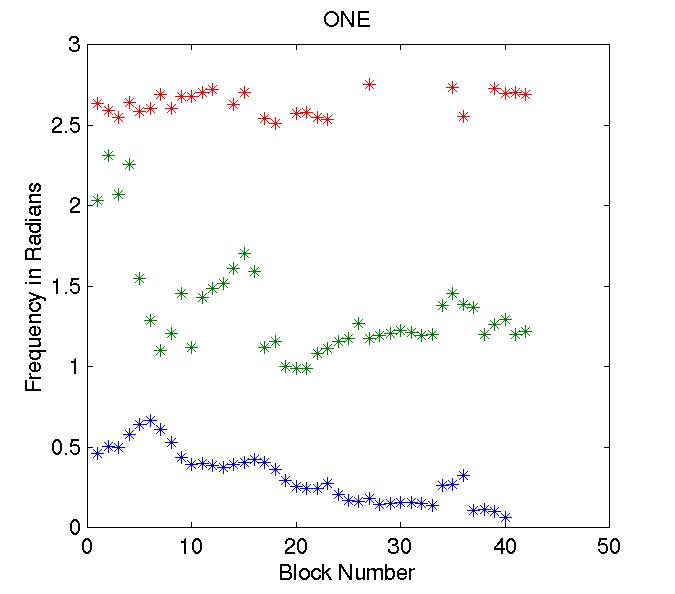
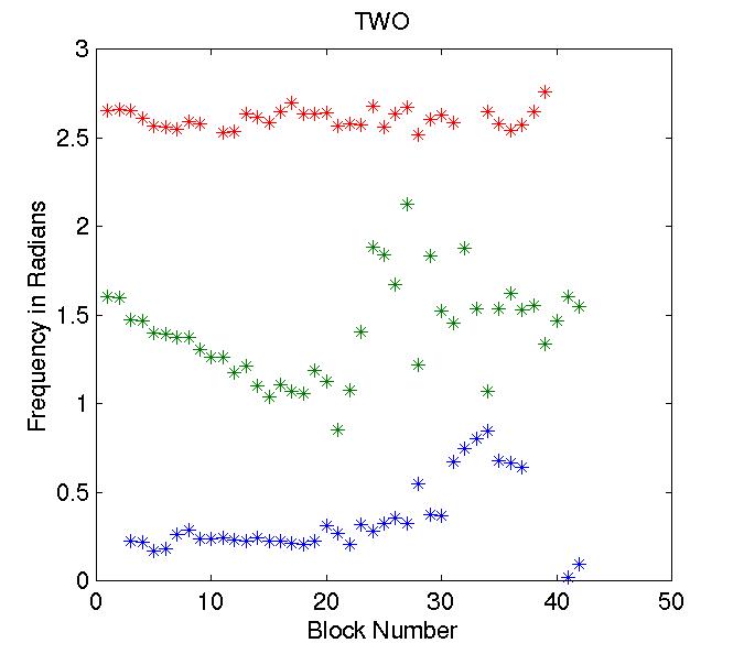
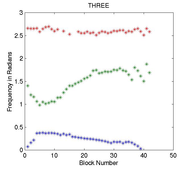
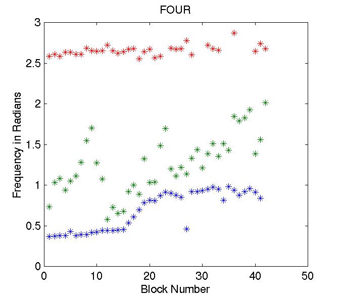
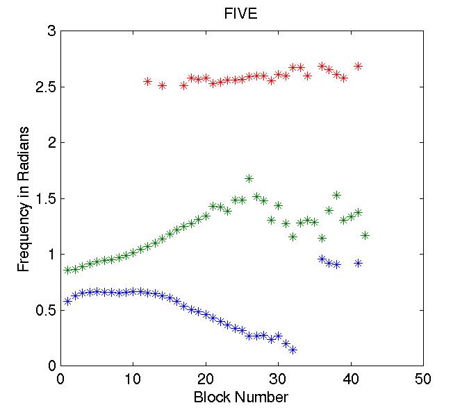
For each window, an AR model was created. The order for the model was chosen to be 8 because this is the optimal value that was determined using the Minimum description length measure. Also this value seems reasonable because in (1) they tracked 3 formant frequencies, and we tracked 3 formant frequencies. An order of 6 was also tested, but with this order, the 3 formant frequencies were not always trackable. Click here for a PSD and a pole zero plot of one of the windows. For each window you have to choose the 3 formant frequencies. A formant trajectory plot is found here. This plot contains the first formant frequency in blue, the second in green, and the third in red. Notice that some of the blocks don't have formant frequencies. This is because for many windows that contained little information (the beginning and the end of the signal) the poles of the AR model were not very close to the unit circle. In other words, the poles were trying the represent a flat spectrum of white noise. If the pole magnitude was less than .8, then it was thrown out. The value .8 was used in (1). Also, if a pole was at zero, or at pie, then it was thrown out. To create the model, 10 realizations were averaged together to form these formant trajectory plots. The matlab program which executes this operation is found at formantmod.m |
|
The program wordrec.m uses the same procedures as above to generate the formant trajectory plots. Once the matrix containing the 3 formant vectors is complete, this matrix is compared to the model for each matrix. The comparison is done by computing the least squared error between each model and the signal to be recognized. In the future, the comparison between the model and the signal would be more accurate if the distance between the two could be determined using a total least squared error.
|
|
The results using this method are found in the Result section. In general, the results are not as good as would be desired. Recognizing the number 4 was particularly hard. Also, the program in kind of an 'ad hoc' way aligns all the words in time and frequency. To get better results, more advanced techniques must be used. Another improvement could be made by manually adapting the models. This would involve removing the points from the plots that visually don't seem to fit. In this way, those points would not be involved in the calculations of the error. This method is more powerful than the power method, and with some fine tuning of the program the error rates could be reduced greatly. |