 |
Beat Detection Algorithm
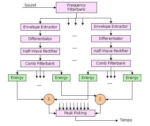
We adapted a beat detection algorithm from the MIT Media Lab to Matlab
for our project. Although the algorithm is quite mathematically
involved, it basically amounts to emphasizing the sudden impulses of
sound in the song and then finding the fundamental period at which
these impulses appear. This is done by breaking the signal into
frequency bands, extracting the envelope of these frequency-banded
signals, differentiating them to emphasize sudden changes in sound,
and running the signals through a comb-filterbank and choosing the
highest energy result as our tempo.
Our algorithm does not account for the possibility of a varying tempo
in a piece of music. It extracts 2.2 seconds of music from the middle
of a song, tempo-analyzes it, and assumes that the tempo found is
associated with the entire piece of music. The sample length, 2.2
seconds, is the minimal amount of information we can work with to have
at least two beats for the slowest tempo we are allowing for,
60 bpm. We are choosing 2.2 seconds rather than 2 seconds to ensure
that the tempo-choosing processing does not exagerrate the energy of
60 bpm. A two second sample could have its beginning and end perceived
as beats by a 60bpm search process. Since 60bpm is our lowest search
tempo, any sample longer than two seconds works fine.
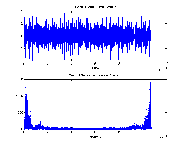
Step 1: Filterbank
The signal is divided up into six separate signals, each consisting of
the frequency content of the original signal from a certain
range. This has the general effect of separating "notes" from
different instrument groups and allowing them to be analyzed
separately. Tempo-analyzing the original signal could be error-prone
due to conflicting downbeats of different instruments. This separation
is performed by taking the FFT of the signal and then taking
appropriate sized chunks of the FFT and assigning them to their
frequency bands. (Chunk length is dependent on both the sampling
frequency and the signal length.) We chose to follow the method
outlined in Scheirer, 1998 and broke our signal into the bands
0-200Hz, 200-400Hz, 400-800Hz, 800-1600Hz, 1600-3200Hz, and finally
3200Hz-Sampling Frequency. This gave us a total of six bands to work
with. The inverse FFT of these signals is taken and their time domain
representation is sent to the smoothing function.
Step 2: Smoothing
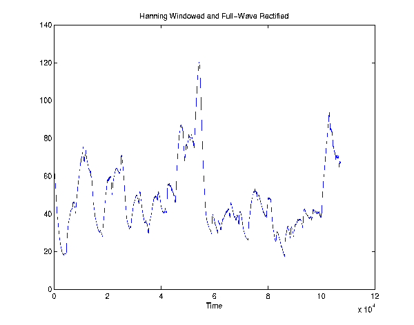
Since we are only looking for the tempo of our signal, we need to
reduce it to a form where we can see sudden changes in sound. This is
done by reducing the signal down to its envelope, which can be though
of as the overall trend in sound amplitude, not the frequencies it
carries. Essentially, we take each of our six frequency-banded
signals and lowpass filter them. To accomplish this we first full-wave
rectified our signals in order to decrease high-frequency content and
so that we would only have to deal with the positive side of the
envelope we were searching for. We then convolved each of our signals
by the right half of a Hanning window with a length of .4
seconds. Again, we chose to do this operation in the by transforming
to the frequency domain, multiplying, and inverse transforming to
decrease computation time. The resulting plots of the frequency-banded
signals definitely correspond to the envelopes of the original
signals.
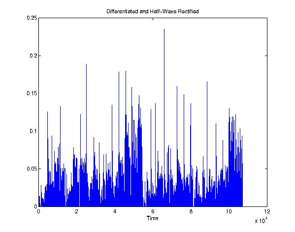
Step 3: Diff-Rect
Now that we have the signals in an enveloped form, we can simply
differentiate them to accentuate when the sound amplitude changes. The
largest changes should correspond to beats since the beat is just a
periodic emphasis of sound. The six frequency-banded signals are
differentiated in time and then half-wave rectified so we can only see
increases in sound. The signals are now ready to be tempo-analyzed.
Step 4: Comb Filter
This is the most computationally intensive step. We need to convolve
the differentiated frequency-banded signals with various comb filters
to determine which yields the highest energy. A comb filter is
basically a series of impulses that occur periodically, at the tempo
you specify. Convolving a comb filter with a total of three impulses
with our signal should give an output that has a higher energy when
the tempo of the comb filter is close to a multiple of that of the
song. This is because the convolving with the three impulse comb
filter just results in an output vector made up of an echoed version
of our original signal. This echoed output will have a higher energy
if the tempo of the signal and comb filter match because it will
result in there being higher peaks (overlap from echo) in the output
which when squared will give a higher energy.
We implemented the comb filter by specifying a range of tempos we
wanted to search for and the resolution or spacing between them. This
established a set of comb filters to convolve with our signal. The FFT
of each frequency-banded signal was multipled by the FFT of each comb
filter and the energy of each of these was taken. Then the energies of
the frequency-bands were summed so that we were left with a vector of
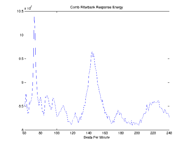
energies of tempos. This output takes the form of a peak at the
fundamental tempo of the song followed by smaller, wider peaks at
multiples of this tempo. We then choose the maximum value of these
energies to be the fundamental tempo of our piece.
Beat Detection Block Diagram
Matlab Code
- filterbank.m -
divides a time domain signal into individual frequency
bands.
- hwindow.m -
rectifies a signal, then convolves it with a half Hanning
window.
- diffrect.m - differentiates a signal, then half-wave rectifies the
result.
- timecomb.m - finds the tempo of a musical signal, divided into
frequency bands.
- control.m - takes in the names
of two .wav files, and outputs their combination--beat-matched, and phase aligned.
Matlab Plots
Step 1:
Filterbank (output of 1 frequency band)
Step 2: Smoothing
Step 3: Diff-Rect
Step 4: Comb Filter
|