We configured our filters for our test patient, Joe.

An audiologist determined that Joe has moderate hearing loss, which is characterized by:

· A Threshold of Hearing at 40 dB
· A Threshold of Pain at 110 dB
· A saturation level (Psat) of 90 dB (where sounds begin to become uncomfortable)
· Difficulty to hear high frequencies

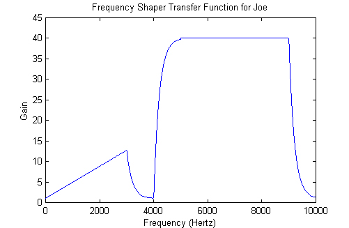
In order to create the gain filter for Joe, we used the concatenation of piecewise functions that change at f = 3000,4000,5000, and 9000 in hertz.

In the actual Matlab function, applySkiSlope, f was mapped to the specific
DFT coefficient that it corresponds to.

Joe's frequency response looks like this:

Here are the signals we used to test our system:

Signal 1 With White Noise

Signal 2 With Noise

The graphs below show what he hears. (Blue is before filtering, Red is after filtering)

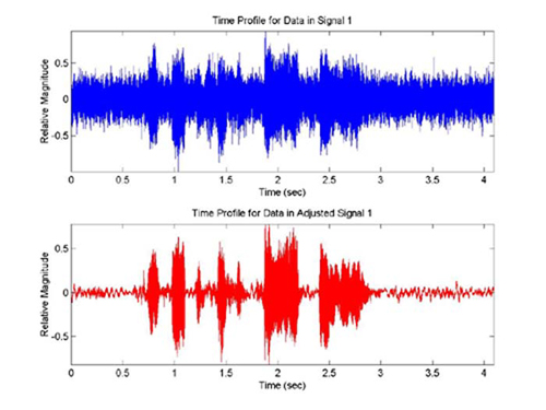
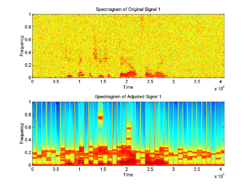
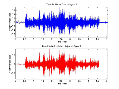
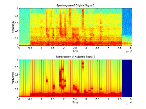
Comparing the graphs of the original signal and the filtered signal, we saw that the amplitude of the noise in the signal was noticeably reduced. We also compared the spectrograms of the two signals and saw that the speech signal was stronger and more recognizable. Our group also listened to the signals and agreed that there was a definite difference.

Here are the signals with reduced noise:

Signal 1 Fixed

Signal 2 Fixed