The problem of speaker identification is one that is rooted in the study of the speech signal. A very interesting problem is the analysis of the speech signal, and therein what characteristics make it unique among other signals and what makes one speech signal different from another. When an individual recognizes the voice of someone familiar, he/she is able to match the speaker's name to his/her voice. This process is called speaker identification, and we do it all the time.

Speaker identification exists in the realm of speaker recognition, which encompasses both identification and verification of speakers. Speaker verification is the subject of validating whether or not a user is who he/she claims to be. In this report we pursue a speaker identification system, so we will abandon discussion of the other topics.

The fundamental assumption that is made in any of these systems is that there are quantifiable features in each person's voice that are unique among individuals and therefore can be measured. The features that we exploit in this project are rooted in the frequency domain, but are not simply Fourier transforms.

A model of speech that is very useful in speaker identification is the following:

That is, the speech signal s(t) is the convolution of a filter h(t) and some signal p(t). h(t), as it turns out, is the impulse response of all the things that get in the way of speech emanating from the lungs, e.g. teeth, nasal cavity, lips, etc. p(t) is the excitation that we refer to as the pitch of speech. p(t) is approximately a periodic impulse train. It is from this that we determine the pitch of speech, where pitch is synonymous with frequency. From our properties of Fourier transforms, we know that in the frequency domain, S(jw) = H(jw)P(jw). This will become very important in a very short while...

The word cepstrum is a play on spectrum, and it denotes mathematically:

where s(n) is the sampled speech signal, and c(n) is the signal in the cepstral domain. We use cepstral analysis in speaker identification because the speech signal is of the particular form above, and the "cepstral transform" of it makes analysis incredibly simple. We see that:

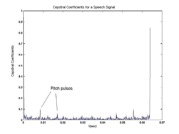
The key is that since the logarithm, though nonlinear, basically just attenuates each spectrum. Since the P(jw) is a pulse train (it's FFT is the same as the signal itself), we can still recover the original pulse train. All we do is look for periodic spikes in the signal, and we have found the pitch of a speaker. Though H(jw) is not a pulse train, we still can use this information. It is always located near the lower part of the cepstrum, and we will use the first twelve cepstral coefficients, as is common in the field.

For humans speakers, Fp, the pitch frequency, can take on values between 80Hz and 300Hz, so we are able to narrow down the portion of the cepstrum where we look for pitch. In the cepstrum, which is basically the time domain, we look for an impulse train. The pulses are separated by the pitch period, i.e. 1/Fp. In order to determine the pitch frequency, we perform the following computation:

We also calculate mel-frequency cepstral coefficients (MCC), delta cepstral coefficients (DMCC), and delta-delta cepstral coefficients (DDMCC). Here we are using the mel scale, which translates regular frequencies to a scale that is more appropriate for speech, since the human ear perceives sound in a nonlinear manner. This is useful since our whole understanding of speech is through our ears, and so the computer should know about this, too. The DMCC's are the derivatives of the MCC's. This sort of tells us how fast a speaker's voice is changing. The DDMCC's likewise tell us something similar to acceleration of pitch. So, it can be seen why these three features were chosen to comprise our feature vectors.

Vector quantization (VQ) is the process of taking a large set of feature vectors and producing a smaller set of feature vectors that represent the centroids of the distribution, i.e. points spaced so as to minimize the average distance to every other point. We use vector quantization since it would be impractical to store every single feature vector that we generate from the training utterance. While the VQ algorithm does take a while to compute, it saves time during the testing phase, and therefore is a compromise that we can live with.

There are a number of clustering algorithms available for use, however it has been shown in [2] that the one chosen does not matter as long as it is computationally efficient and works properly. A clustering algorithm is typically used for vector quantization, and the words are, at least for our purposes, synonymous. Therefore, we have chosen to use the LBG algorithm proposed by Linde, Buzo, and Gray, since it was provided in the VOICEBOX speech processing toolkit for MATLAB.

After taking our enormous number of feature vectors and approximating them with our smaller number of vectors, we file away these vectors into our codebook and refer to them as codewords.

After quantizing a speaker into his/her codebook, we need a way to measure the similarity/dissimilarity between and two users. It is common in the field to use a simple Euclidean distance measure, and so this is what we have used.

We follow the algorithm proposed in [1] to weight distances so as to increase the likelihood of choosing the true speaker. This algorithm, basically, reflects the greater importance of unique codewords as opposed to similar ones, so as to increase inter-speaker variability. This is a very important portion of our system, since the qualities that we are looking for in the speech signals are very subtle. Likewise, the algorithm also decreases the importance of similar codewords, since they yield no distinguishing information.